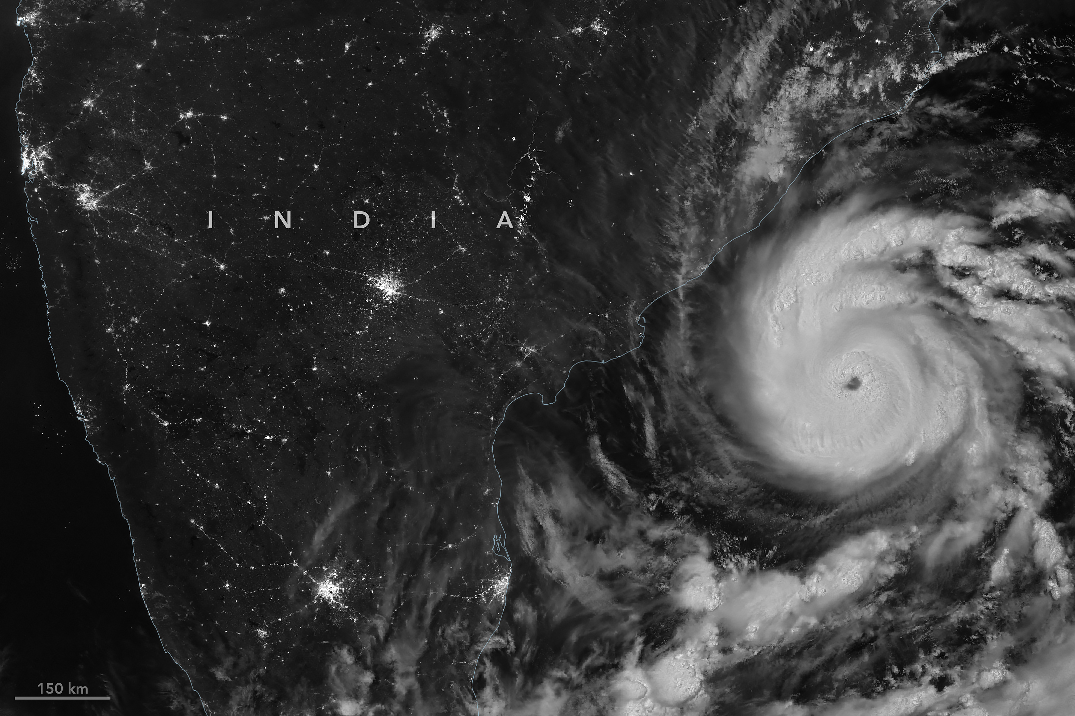
The first named storm of the 2026 North Indian Ocean cyclone season—Arnab (pronounced Or-nab)—emerged in the Bay of Bengal on October 25, a rather late start for a basin that typically produces named cyclones in April or May.
When the VIIRS (Visible Infrared Imaging Radiometer Suite) on NOAA-20 captured this nighttime image at 20:12 Universal Time on October 26 (1:42 a.m. India Standard Time on October 27), the storm had sustained winds of about 140 kilometers (85 miles) per hour, according to the India Meteorological Department (IMD).
When Arnab made landfall on the Andhra Pradesh and Yanam coast early on October 28, sustained winds were 130 kilometers per hour. IMD categorizes a storm that strength as a “very severe cyclonic storm,” which is similar to a Category 1 storm on the Saffir-Simpson hurricane wind scale. It made landfall between Bapatla and Visakhapatnam, a heavily settled area home to large cities, farmland, and fishing communities.
Arnab caused extensive damage, uprooting trees, inundating crops and homes, limiting fishing operations, and disrupting transportation and power networks, according to news reports. Prior to landfall, Indian authorities had evacuated tens of thousands of people from vulnerable coastal areas.
The storm comes in the midst of an El Niño, a climate pattern marked by warmer-than-normal water temperatures in parts of the equatorial Pacific that emerges roughly every two to seven years. The changed ocean conditions can influence the atmosphere in ways that alter global weather patterns and change the distribution of rainfall, winds, tropical cyclones, fires, floods, and other phenomena.
In the Bay of Bengal, for instance, some research indicates that altered environmental conditions during an El Niño are associated with a reduction in tropical cyclone activity. The ocean basin sees both less frequent and less intense tropical cyclones during El Niño years, researchers have found.
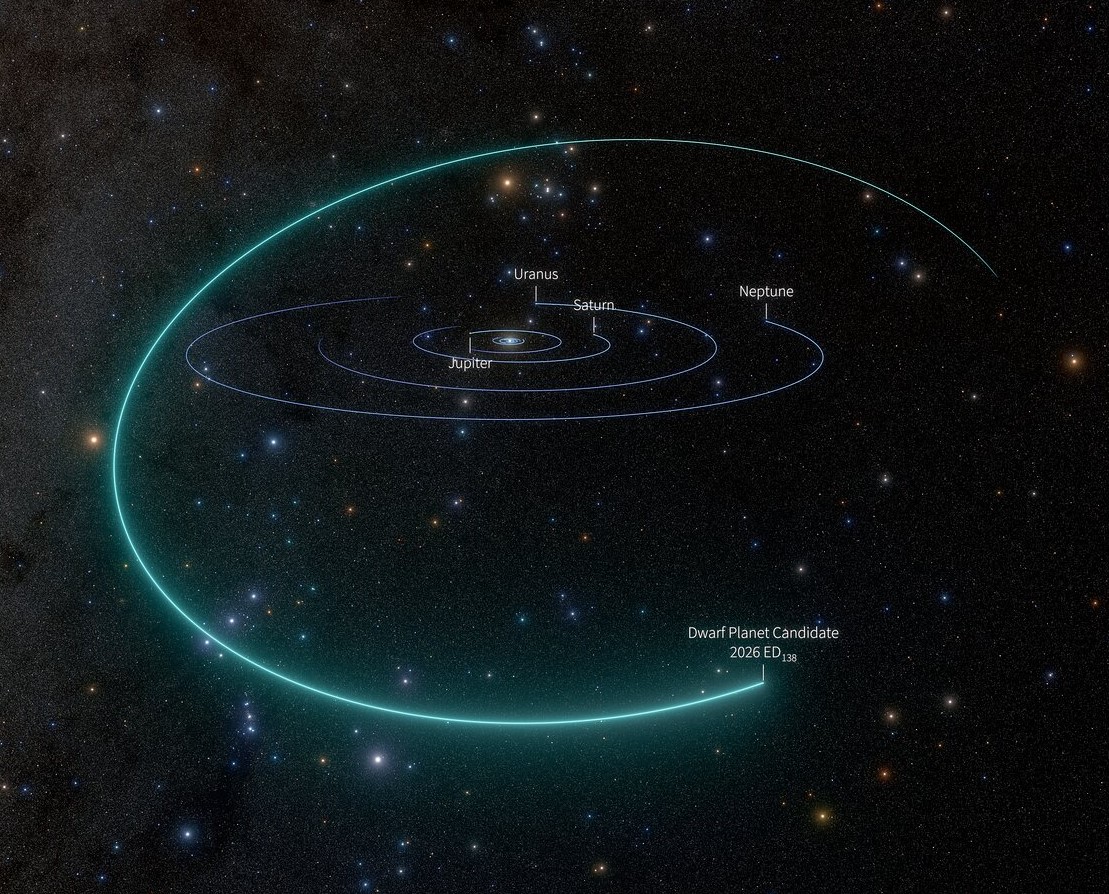
A visualization shows the orbital path of the dwarf planet candidate 2026 ED138 in relation to the orbits of the solar system’s larger planets. Click on the image for a larger version. (Credit: NSF-DOE Vera C. Rubin Observatory / NOIRLab / SLAC /AURA / R. Proctor)
Astronomers sorting through data from the Vera C. Rubin Observatory in Chile have found an icy world that has a good chance of joining Pluto in the solar system’s retinue of dwarf planets.
University of Washington astronomer Mario Jurić joined the astronomer who made the discovery, Matthew Holman of the Harvard & Smithsonian Center for Astrophysics, to announce the findings today at a meeting of the American Astronomical Society’s Division for Planetary Sciences in Spokane, Wash.
Jurić, the Rubin team’s solar system lead scientist, said the observatory’s capabilities made it possible to detect and characterize the new dwarf planet candidate, known as 2026 ED138.
“Rubin is giving us an unprecedented capacity to explore the sky through a combination of speed, depth, and precision,” Jurić said in a news release. “And the discovery is just the beginning: Once we identify a new object, we can search back months, and sometimes even decades, finding it in images where nobody knew to look. This ability to both discover and ‘precover’ objects is transforming how quickly and accurately we can determine their orbits and understand the distant solar system.”
2026 ED138 traces a tilted orbital path that takes it well beyond Pluto, the solar system’s best-known dwarf planet. It’s currently at a distance of 46 astronomical units, where 1 AU equals the average distance between Earth and the sun. Pluto, by comparison, is currently about 40 AU from the sun.
Astronomers suspect ED138 formed billions of years ago closer to the sun before being flung into a wider orbit by gravitational interactions with Neptune.
Based on an analysis of its distance, brightness and assumed composition, ED138 is thought to be somewhere between 600 and 1,500 kilometers (373 to 932 miles) in diameter. At that size, an icy object should possess enough gravity to pull itself into a round shape — satisfying the primary physical criterion for a dwarf planet.
Rubin’s researchers analyze the data from those scans to find objects of interest — ranging from asteroids to gamma-ray bursts — and track them over time. On Oct. 13, Holman was running data through a search code that he developed with Kevin Napier, a colleague at the Center for Astrophysics. ED138 stood out due to its exceptional size and brightness.
“My first reaction was one of excited disbelief,” Holman said. “Objects like this are very rare, so I immediately started checking whether I or the code had done something wrong.”
To confirm the discovery, Holman, Jurić and their colleagues found 30 archived observations of ED138 dating back to March 4. The Asteroid Institute’s ADAM Precovery service found still more images of the object, going back to 2016, in the archives of a different astronomical survey.
The precovery data confirmed that ED138 was a special case.
“Finding an object this big, roughly 1,000 kilometers across, is something that happens maybe once in a generation,” Jurić said. “It’s the largest trans-Neptunian object found in about 20 years, and Rubin turned it up while we were still commissioning the telescope.”
In 2006, the International Astronomical Union defined dwarf planets as planetary objects that are big enough to crush themselves into a roundish shape — technically speaking, into a state of hydrostatic equilibrium — but not big enough to clear their orbital neighborhood.
So far, the IAU has classified five solar system objects as dwarf planets — including Ceres in the main asteroid belt, plus Pluto, Eris, Haumea and Makemake in the region beyond Neptune. 2026 ED138 joins a host of other celestial objects that are thought to be dwarf planets but haven’t yet been added to the IAU’s official list.
“The official list hasn’t moved since 2008,” Jurić told GeekWire in an email. “I’m not sure if there’s an active process that reviews candidates, and what are the timelines.”
Jurić and his colleagues hope additional observations will boost ED138’s chances of attaining true dwarf planethood.
“The next step in building the case would be to prove it’s round (in hydrostatic equilibrium),” he wrote. “The means to do that would be directly through occultations (and there’s a good chance of that, given it’s in a dense stellar field), and then thermal measurements plus modeling and light curves (or the absence of variability).”
Some 27 million years ago, a volcano in what’s now southeastern Arizona unleashed a spectacular series of eruptions, strewing more than 1,000 times as much volcanic material across the landscape as Mount St. Helens did in 1980.
The explosive eruptions blanketed the region, part of the Chiricahua Apache Nation’s traditional lands, with ash and pumice. Layered into this were massive pyroclastic flows that hardened into deposits of welded rhyolitic tuff that in some areas were nearly 1,600 feet (500 meters) thick, about three times the height of the Washington Monument. As the magma chamber emptied, the ground above it collapsed, leaving a gaping depression—the Turkey Creek caldera—that was roughly 12 miles (19 kilometers) wide and 4,900 feet (1,500 meters) deep.
An array of geologic processes, including erosion and weathering, gradually sculpted the welded layer of tuff into the collection of dramatic spires, hoodoos, and canyons that visitors to the caldera area encounter today.
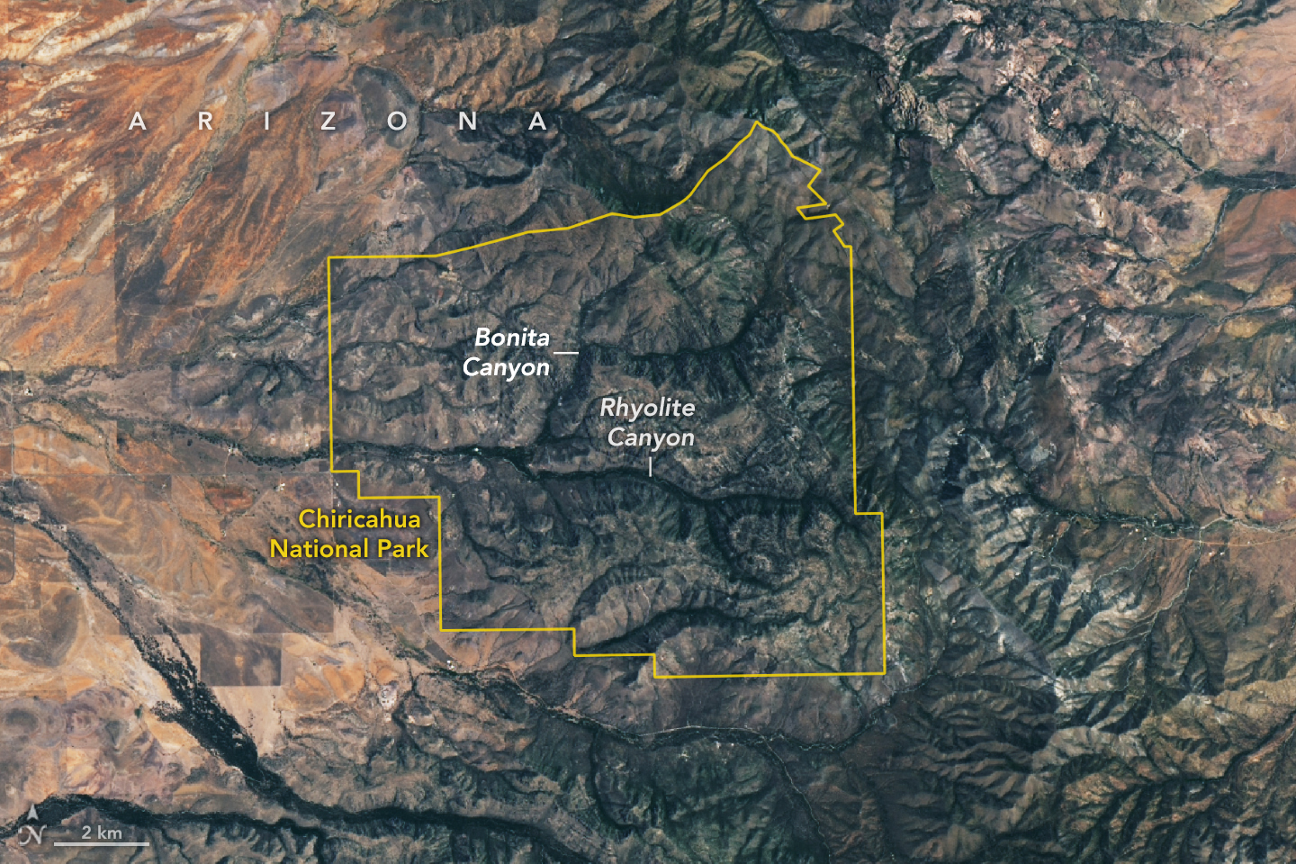
The area was designated a national monument in 1924 to preserve its remarkable geology. In October 2026, it was redesignated as Chiricahua National Park (pronounced cheery-cow-ah). The OLI (Operational Land Imager) on Landsat 9 captured this cloud-free image of the new national park on July 2, 2026.
Individual rock spires are too small to distinguish, but the eroding rhyolitic tuff landscape appears gray. Stream valleys dense with trees and other vegetation, including Rhyolite Canyon and Bonita Canyon, snake across the landscape. With four biogeographic regions converging in the park—the Sonoran Desert, the Chihuahuan Desert, the Rocky Mountains, and the Sierra Madre—it is a haven of plant diversity.
Among the 1,000 species growing within the park’s varied desert, grassland, chaparral, deciduous forest, and coniferous forest ecosystems are agaves, prickly pear cacti, yuccas, manzanita, pine, fir, cypress, sycamore, juniper, and oak. The park’s location within the Chiricahua Mountains puts it among several “sky islands” in Arizona—isolated mountain ranges that emerge from the surrounding desert “sea.” According to the National Park Service, the range’s highest point (outside the park) rises 2,986 meters (9,795 feet) above sea level, more than 1,800 meters above the surrounding valley.
NASA Earth Observatory image by Lauren Dauphin, using Landsat data from the U.S. Geological Survey. Story by Adam Voiland.
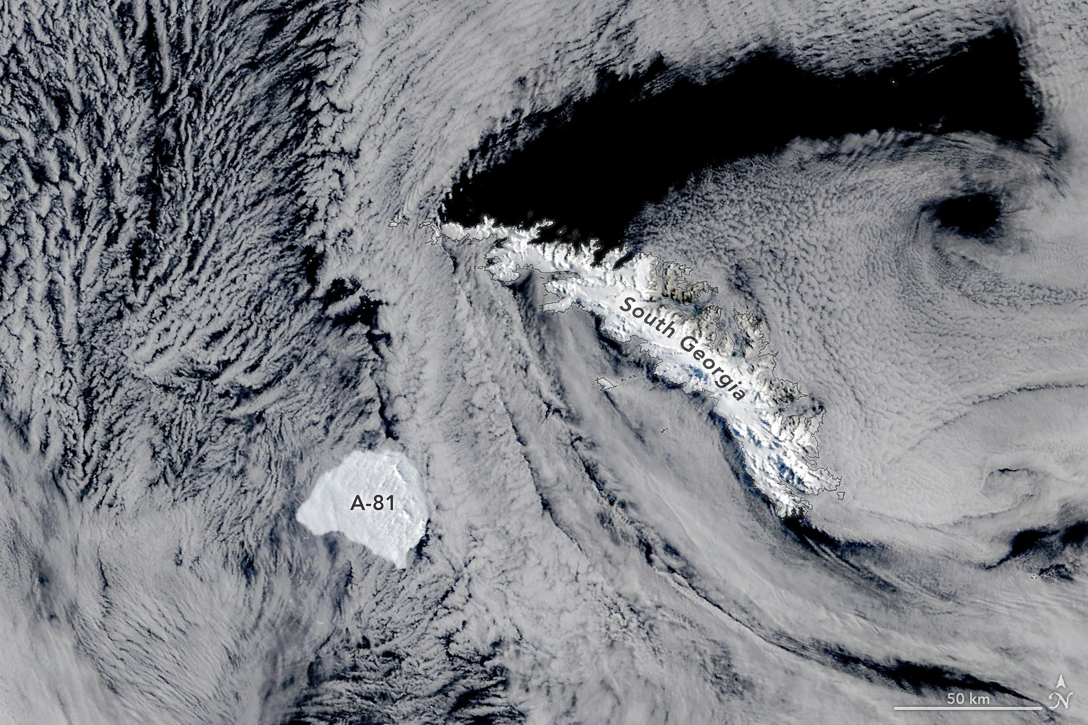
Iceberg A-81 slows its drift near the edge of South Georgia’s shallow underwater shelf in this image, acquired on October 20, 2026, by the MODIS (Moderate Resolution Imaging Spectroradiometer) on NASA’s Terra satellite.
NASA Earth Observatory/Michala Garrison
Some Antarctic icebergs linger close to home for decades, running aground near the ice shelves that spawned them or circling partway around the continent on coastal currents. Others, like Iceberg A-81, make a faster exit, heading north out of the Weddell Sea along a route well-traveled by the region’s bergs.
Fast is relative, though. After breaking from the Brunt Ice Shelf in January 2023, the roughly 1,550-square-kilometer (600-square-mile) berg spent more than three years in the Weddell Sea, carried along the coast by the clockwise-flowing Weddell Gyre. By May 2026, it reached the tip of the Antarctic Peninsula. It then moved north into the Scotia Sea, and by late October 2026, it approached the remote island of South Georgia in the South Atlantic Ocean, 2,300 kilometers (1,400 miles) north-northwest of the Brunt Ice Shelf.
This image, acquired by the MODIS (Moderate Resolution Imaging Spectroradiometer) on NASA’s Terra satellite, shows the berg on October 20. In the days before, its progress slowed noticeably, and it appeared to be bumping along the edge of the island’s underwater shelf, according to Jan Lieser of Australia’s Bureau of Meteorology and Christopher Shuman of the University of Maryland (retired). South Georgia has slowed and even stopped icebergs before. In 2025, for instance, Iceberg A-23A ran aground on the shelf and later broke apart.
Though Iceberg A-81 was a steadfast traveler once it broke free, it took its time in becoming an iceberg in the first place. For about 35 years, one of the Brunt Ice Shelf’s rifts known as Chasm 1 was relatively stable. Then, around 2012, it began growing again, and by 2019, it was advancing quickly enough that a break seemed imminent. But the floating glacial ice held on for several more years until finally, in January 2023, the berg let go.
Calving is a normal part of the life cycle of ice shelves, but scientists keep a close eye on Brunt, which has recently shed several large icebergs in quick succession and is home to the British Antarctic Survey’s Halley Research Station, a major base for Earth, atmospheric, and space science research since the 1950s. Besides A-81, the ice shelf calved Iceberg A-74 from the North Rift in 2021 and Iceberg A-83 from the Halloween Crack in 2024. A-74 has since broken up, while A-83 remains intact and is trailing A-81 northward, along with a handful of other icebergs that appear to be clearing out of the Weddell Sea.
NASA Earth Observatory image by Michala Garrison, using MODIS data from NASA EOSDIS LANCE and GIBS/Worldview. Story by Kathryn Hansen.
A map depicts vegetated parts of Earth’s land surfaces from September 29 to October 4. Vegetation color is depicted on a spectrum ranging from dark green to light yellow to dark red. The largest patches of red vegetation appear in Alaska, northern Canada, Mongolia, and Russia. Smaller patches of red are visible in Australia.
NASA Earth Observatory / Lauren Dauphin
A similar global map depicts the redness of vegetation from October 5 to 11. The reddest areas have shifted equatorward, with more color visible in the Mid-Atlantic, the U.S. Southeast, southern Russia, China, and Mongolia.
NASA Earth Observatory / Lauren Dauphin
September 29 to October 4
October 5 to 11
These maps show the redness of vegetation as measured by the OCI (Ocean Color Instrument) on the PACE (Plankton, Aerosol, Cloud, ocean Ecosystem) satellite in September and October 2026. Red foliage appears to peak in New England, northern Canada, and northern Russia from September 29 to October 4, then spreads southward into the Mid-Atlantic, Mongolia, and northern China from October 5 to 11 (right).
The Japanese tradition of momijigari, or “red leaf hunting,” stretches back more than a millennium, as evidenced by ancient poems describing journeys to admire fall foliage. In America, mentions of foliage trips began appearing in the historical record in the 19th century, around the time artists and poets such as Frederic Church and Emily Dickinson celebrated autumn color in depictions of the Northeast.
Modern-day leaf peepers have a new way to track and savor the seasonal phenomenon. The hyperspectral OCI (Ocean Color Instrument) on NASA’s PACE (Plankton, Aerosol, Cloud, ocean Ecosystem) satellite observes the planet’s oceans and vegetation daily at 286 spectral bands. Among this array are a few groups of wavelengths that allow scientists to track subtle changes in leaf pigments key to fall foliage displays, including anthocyanins (reds), carotenoids (yellows and oranges), and chlorophylls (greens).
NASA scientists can track fall color by measuring how much red, orange, and yellow forests show compared with green. Tracking the ratio over time reveals where leaves are changing and when color peaks. The maps above show vegetation “redness” from September 29 to October 4 (left) and October 5 to 11 (right). Areas shown in green have values near 1, meaning the satellite detects about as much red as green, and most leaves have not yet turned. Areas shown in light yellow and red have higher values, indicating progressively more red pigment relative to green.
The satellite detected particularly high levels of redness in parts of northern and eastern Russia, northern Alaska, and northern Canada from September 29 to October 4. In New England and upstate New York, redness began to fade during the week of October 5 to 11, even as it spread across much of the Midwest and the Mid-Atlantic. (Not all the yellows and reds on the maps represent fall colors. Crops in some agricultural areas, for instance, show high anthocyanin levels as they age and after they are harvested. Also, in some regions, clouds produce what appear to be gaps in the vegetation.)
Seeing Red in Vermont
Many of the reddest areas—such as the Adirondacks in New York, the Green Mountains in Vermont, and the White Mountains in New Hampshire—have large numbers of sugar maples (Acer saccharum) and red maples (Acer rubrum), deciduous trees that turn a brilliant shade of crimson in the fall. Blueberries, bilberries, sedges, mosses, and grasses likely contribute to the intense reds detected in marshy tundra areas in northern Alaska, Canada, and Russia.
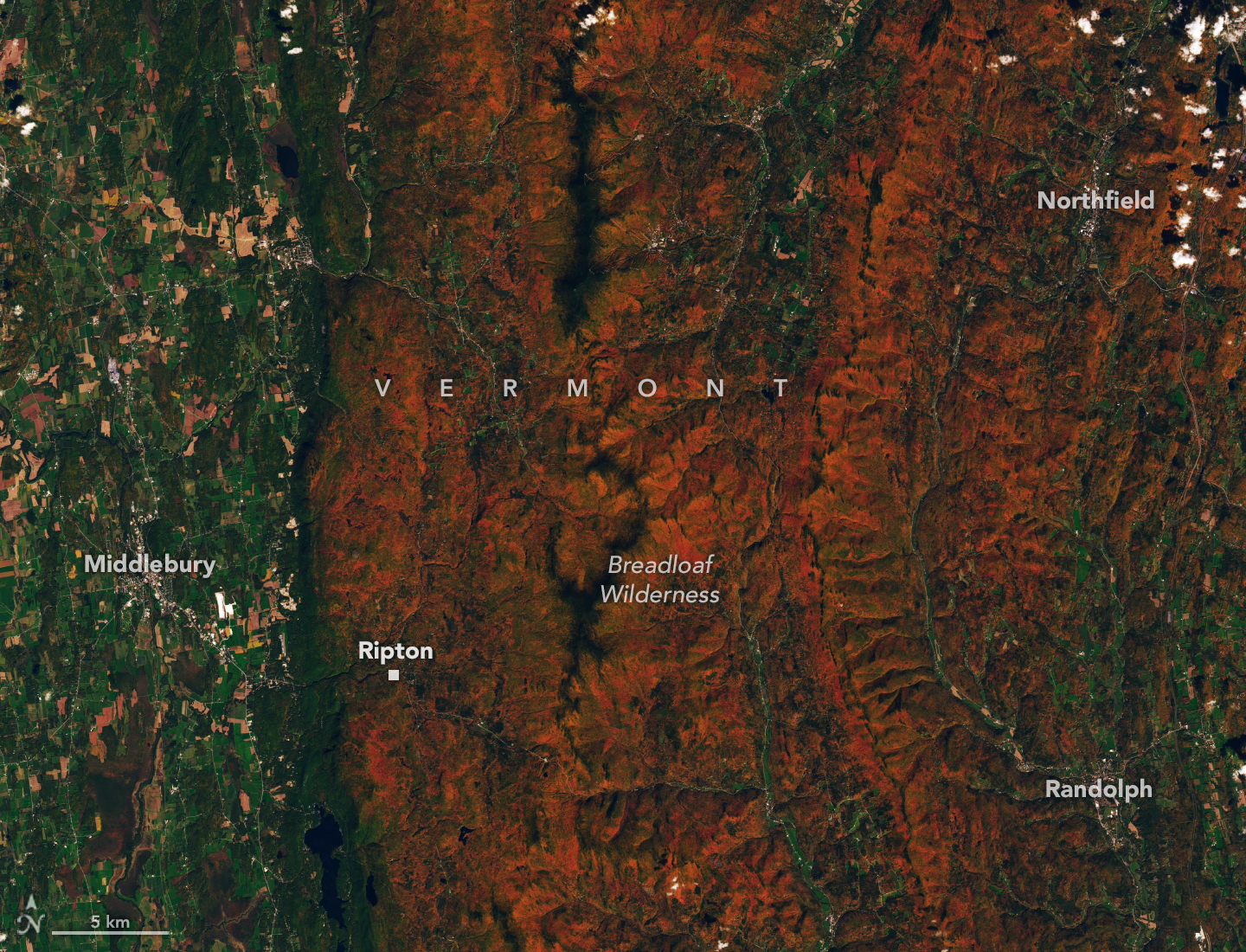
Red and orange hues cover the forested ridges of central Vermont, while river valleys and lower-elevation areas are still green. The OLI (Operational Land Imager) on Landsat 9 captured this image on October 3, 2026.
NASA Earth Observatory / Lauren Dauphin
The OLI (Operational Land Imager) on Landsat 9 captured an image (above) of intensely red foliage around Ripton, Vermont, on October 3, 2026, around the peak of redness in the region. Poet Robert Frost, author of “October,” “The Road Not Taken,” “Nothing Gold Can Stay,” and several other poems that evoke fall foliage, kept a summer home and farm in Ripton and taught at Middlebury’s Bread Loaf School of English.
Some other satellites with hyperspectral sensors can measure fall foliage pigments in a way that is similar to PACE, but only in more localized areas and less frequently. PACE is the first satellite capable of measuring all three key leaf pigments—anthocyanins, carotenoids, and chlorophylls—across the entire planet every day or two.
“It’s the ability to collect time-series data of anthocyanins and carotenoids everywhere on Earth repeatedly that is game-changing,” said Karl Huemmrich, a vegetation scientist with the Goddard Earth Sciences Technology and Research II center at the University of Maryland, Baltimore County. Huemmrich, who is also a member of the PACE science team, was eager to work with the satellite because of OCI’s broad swath and short revisit time. “The time-series data allow us to determine peak redness and yellowness anywhere on Earth,” he said.
In the fall, leaves change colors as they lose chlorophyll, a green molecule that plants use to synthesize food. Since chlorophyll is not a stable compound, plants must continuously synthesize it, a process that requires ample sunlight and warm temperatures. As temperatures decrease and days shorten in autumn, levels of chlorophyll drop, causing greens to fade and presenting an opportunity for carotenoids and anthocyanins to show their colors.
Observing Leaves in a Canopy Near You
As part of the ongoing North American Phenology Campaign run by the Global Learning and Observations to Benefit the Environment (GLOBE) program, NASA data scientist Skye Caplan has been posting weekly foliage maps of vegetation redness. The maps show waves of red emerging in the high latitudes in August and shifting equatorward in September and October. The PACE team is asking the public to submit photos of fall foliage to help scientists “ground truth” the satellite observations and better understand how various factors influence vegetation color.
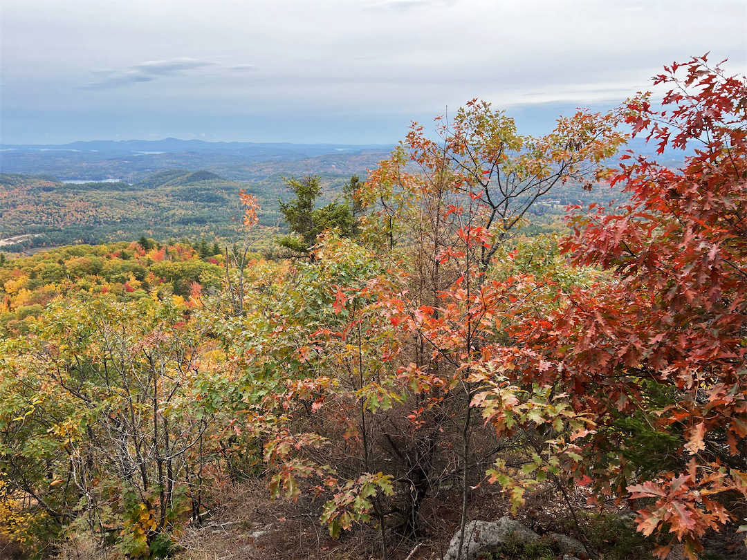
Fall foliage sprinkles a forested New England landscape in a photo taken in Meredith, New Hampshire, on October 11, 2026, by a participant in GLOBE’s North America Phenology Campaign.
GLOBE
“Changes in pigments can also occur when vegetation is stressed due to drought or insect damage,” said Caplan. She noted that changes like these likely help explain why PACE measures high levels of redness in agricultural regions of Brazil, Australia, and Canada that don’t track closely with broader seasonal changes.
“The more photos we can get from the ground, the better,” Caplan said. Ground photos help scientists refine PACE’s observations of vegetation color, which the team hopes will eventually support several lines of research. These include how the timing of spring greening and fall senescence is changing, how vegetation changes affect the global carbon cycle, and how leaf color influences wildfire risk. Scientists also want to know whether PACE can detect early warning signs of drought, insect infestations, and plant disease.
People can participate in the GLOBE campaign even if they live in an area without dense forests or picturesque fall foliage displays. Scientists also want ground observations of shrubs, grasses, wildflowers, evergreens, crops, and other vegetation. But when it comes to “red leaf hunting,” don’t delay, Caplan said. “Color changes happen kind of slowly, then all at once, and then they’re gone.”
NASA Earth Observatory images by Lauren Dauphin, using PACE data courtesy of Skye Caplan/NASA’s Goddard Space Flight Center and Landsat data from the U.S. Geological Survey.Photo courtesy of the GLOBE Program. Story by Adam Voiland.
NASA’s Swift Mission Ends, Leaves Behind Scientific Bonanza
NASA’s Neil Gehrels Swift Observatory has ended its science mission now that the spacecraft is orbiting less than 171 miles (275 kilometers) above Earth’s surface. The greater atmospheric drag at this height prevents the satellite’s telescopes from steadily gazing at their astronomical targets.
Swift conducted its final observation on Oct. 20. It is expected to re-enter the atmosphere in the next few weeks.
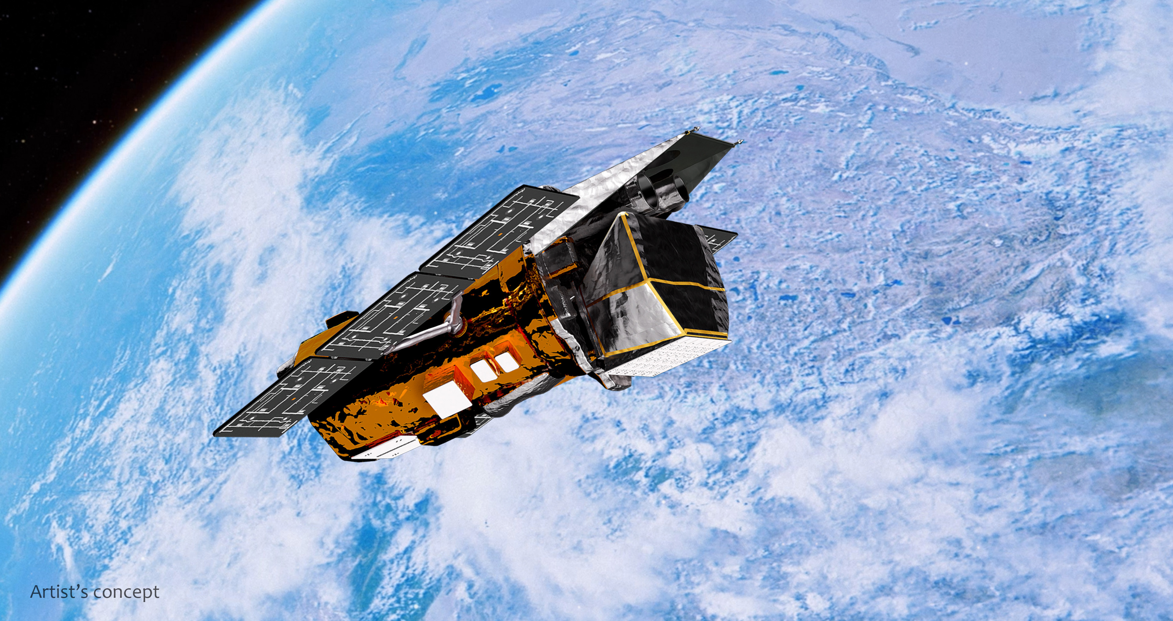
NASA’s Neil Gehrels Swift Observatory orbits above Earth in this artist’s concept.
NASA’s Goddard Space Flight Center Conceptual Image Lab
“Swift delivered an incredible, lasting return on investment for the nation, designed for a two-year primary mission but productive for more than 10 times as long,” said Shawn Domagal-Goldman, director, Astrophysics Division at NASA Headquarters in Washington. “In that time, Swift played a major role in advancing our understanding of the changing universe and was part of a revolution in astrophysics that showed how critical rapid-response observations are to the entire community. To support rapid response to cosmic events in a post-Swift world, we’re exploring our ability to use and augment NASA’s fleet of existing space telescopes, from fast-to-orbit commercial capabilities to efficient, innovative new missions. And Swift leaves us with an extraordinary archive of multiwavelength observations that will fuel new discoveries for decades more.”
In its storied career, Swift has observed more than 2,000 gamma-ray bursts, the most powerful explosions in the cosmos. It has studied more than 1,400 supernova explosions, witnessed stars shredded by black holes, monitored active galaxies, conducted an all-sky X-ray survey, studied asteroids and comets, and more. Swift data has contributed to about 7,000 published scientific papers.
“Swift was designed as a satellite dedicated to studying gamma-ray bursts, outbursts that came and went so quickly that no one could target them with large telescopes to learn more,” said S. Bradley Cenko, the mission’s principal investigator at NASA’s Goddard Space Flight Center in Greenbelt, Maryland. “Swift needed to detect and locate gamma-ray bursts, communicate their position to other observatories, and then swing its telescopes around to image the burst locations before their afterglows faded out. This typically took Swift about a minute to do.”
Led by its first principal investigator, Neil Gehrels, Swift was born as a multiwavelength observatory, with co-aligned Optical/Ultraviolet and X-ray telescopes that could quickly image and refine a burst’s position. The mission launched into orbit on Nov. 20, 2004, and went to work the following month. In 2018, NASA renamed the mission to honor Gehrels following his death.
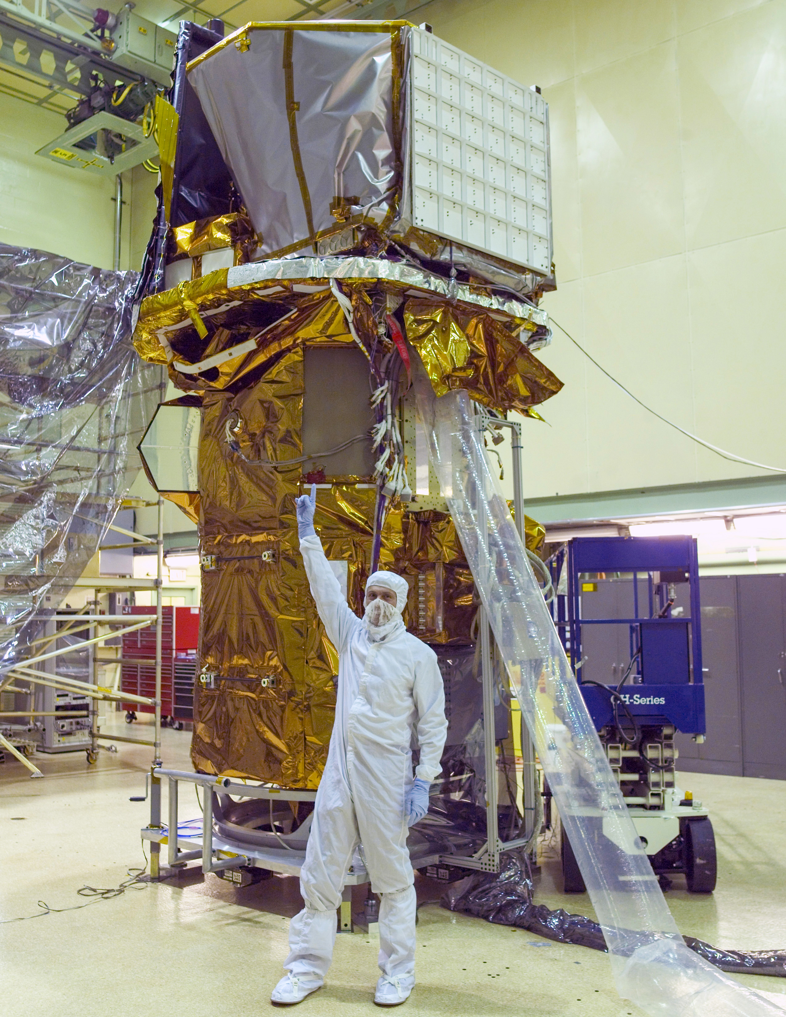
The completed Swift spacecraft is seen in a clean room at NASA Goddard on Sept. 9, 2003. In front of it, Neil Gehrels, the mission’s first principal investigator, points toward the instruments at the top.
NASA
Speed was especially important for an elusive population called short gamma-ray bursts, which reach peak brightness in less than two seconds. Until Swift, it had been impossible to locate these bursts rapidly and precisely enough to observe their afterglows. In May 2005, Swift achieved this milestone with GRB 050509B, which lasted just 0.03 seconds. Swift turned to the burst fast enough to detect 11 X-ray photons, making this the first short burst with a detected afterglow. These observations validated long-standing theoretical models, showing that short gamma-ray bursts likely come from mergers of two neutron stars — objects with the mass of the Sun that have been crushed to the size of a city.
Another factor led to Swift’s success as a kind of astronomical multitool. Its flexible planning system enabled astronomers to request “target-of-opportunity” observations that could be commanded from the ground in as little as a few minutes, or to set up monitoring programs for observing specific sources lasting from as little as a few minutes to months. The system could schedule up to 75 independent targets a day.
“The unique speed of response of the Swift hardware, the extraordinary success of the rapid mission operations, and the closely knit teamwork of the Swift Flight and Science Operations teams placed Swift at the crossroads of burgeoning areas of research,” said John Nousek, the mission’s operations director and professor of astronomy and astrophysics in the Eberly College of Science at Penn State in University Park, Pennsylvania.
The Swift archive contains nearly 22 years of brightness measurements of all kinds of cosmic outbursts, multiwavelength spectra, more than 1.5 million images from its Ultraviolet/Optical Telescope, and much more. The full dataset, publicly available as part of NASA’s commitment to open, gold standard science, spans approximately 12 terabytes, the storage equivalent of about 600 high-definition movies.
As part of the agency’s previous planning for Swift’s end of mission, NASA will continue to prioritize finding new options to react rapidly to cosmic events, using current missions to help fill the gap in the meantime.
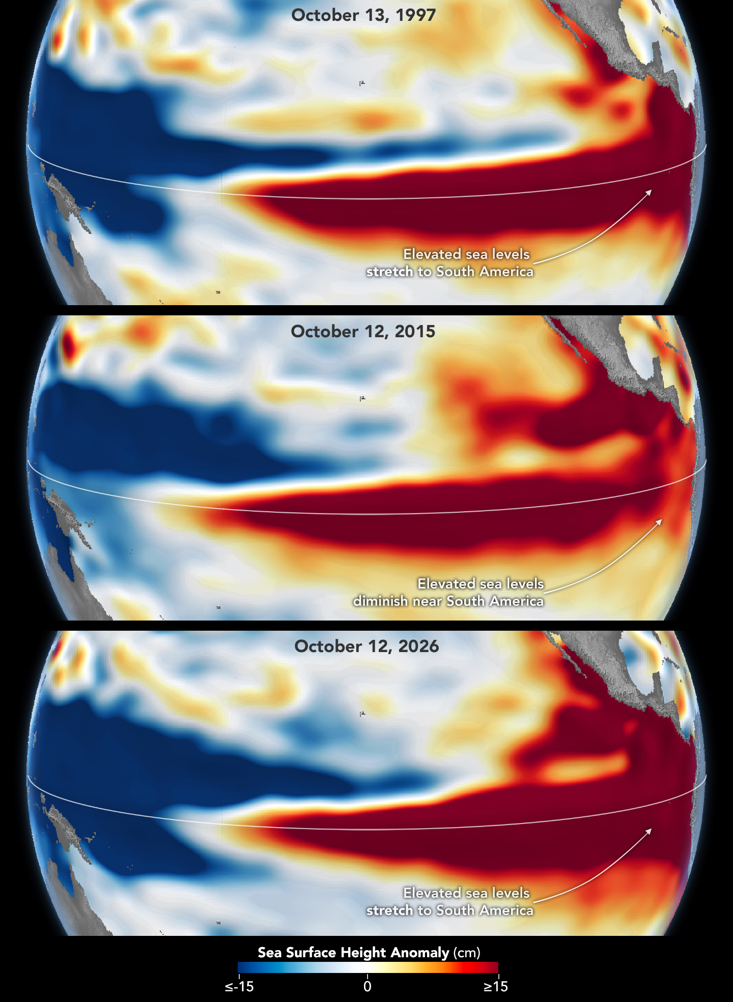
Sea levels are higher than normal across the central and eastern equatorial Pacific in October 2026 (right), a hallmark of El Niño. The pattern closely resembles October 1997 (left), during another one of the strongest El Niño events in the satellite altimetry record.
NASA Earth Observatory / Lauren Dauphin
october 13, 1997
october 12, 2026
October 13, 1997 – October 12, 2026
Sea levels are higher than normal across the central and eastern equatorial Pacific in October 2026 (right), a hallmark of El Niño. The pattern closely resembles October 1997 (left), during another one of the strongest El Niño events in the satellite altimetry record. Maps by NASA Earth Observatory/Lauren Dauphin using altimetry data provided by NASA/JPL-Caltech.
El Niño is part of a natural climate pattern that occurs roughly every two to seven years, bringing warmer-than-normal water to parts of the equatorial Pacific. The most recent very strongEl Niño events, in 1997-98 and 2015-16, upended weather patterns. Impacts spanned the planet, from fires in Indonesia and the Amazon, to crop failures due to drought in southern Africa, to heavy rain and coastal flooding in Southern California. The current El Niño rivals these past heavyweights.
Every El Niño grows from a feedback loop between the atmosphere and the ocean. Trade winds normally keep warm water piled up in the western Pacific, where it stands higher than in the east. When those winds weaken, that warm water begins to pulse eastward, which further weakens and sometimes reverses the winds, allowing even more warm water to move east. The cycle intensifies as waters continue to warm and pile up in the central and eastern Pacific.
But each El Niño has its own character, shaped by where in the Pacific the warmth builds and how the atmosphere responds. “The search for the ‘typical’ El Niño is very elusive,” said Josh Willis, project scientist for sea level missions at NASA’s Jet Propulsion Laboratory (JPL). “They’re all different in terms of where they land and how their impacts play out.”
Altimetry satellites can track those differences by measuring the height of the sea surface. Because water expands as it warms, higher-than-normal sea levels in the central and eastern equatorial Pacific signal the buildup of heat associated with El Niño. The maps above depict sea surface height anomalies across the Pacific Ocean on October 13, 1997 (left), and on October 12, 2026 (right). Data are from the TOPEX/Poseidon satellite and the Sentinel-6 Michael Freilich satellite, respectively, and were processed by scientists at JPL.
Shades of red indicate where sea levels were higher than average. Normal sea level conditions appear white, and lower areas are blue. Signals related to seasonal cycles and long-term trends have been removed to highlight sea level anomalies associated with El Niño and other short-term natural phenomena.
“What’s unique about altimetry is that we have a 35-year record from nearly identical satellites flying almost the same ground track, with each mission overlapping the next,” Willis said. “That lets us look back in time and compare this El Niño to what happened in 1997. And right now, this one is on track to be even bigger.”
Compared with the 1997-98 event, El Niño in 2026 came on much more suddenly. But as of October, the two events appear similar in character—the tilt of sea level (low in the west and high in the east) and high, warm water extending all the way to South America—so Willis thinks the impacts could be similar as well. In 1997-98, that meant, for instance, lots of rain in California and across the southern tier of the U.S.
The 2015-16 El Niño was also very strong, as elevated sea levels in October 2015 (middle) show. But its pattern differed from those in October 1997 (top) and October 2026 (bottom): less of the elevated water reached the coast of South America, which contributed to different weather patterns that year.
The 2015-16 El Niño was another heavy hitter but differed in its character. Sea surface height anomalies on October 12, 2015, based on altimetry data from the Jason-2 satellite, are shown above in context with maps from around the same time in 1997 and 2026. In 2015, the exceptionally warm, high water along the equator didn’t push up against South America to the extent it did in the other years. Rainfall impacts that winter concentrated more over Central America and the southeastern U.S., with significant flooding in Mexico.
NOAA’s El Niño outlook on October 8, 2026, called for an 83 percent chance of a strong-to-very strong El Niño through the first three months of 2027. But exactly how the impacts will play out in winter 2026-27 and beyond remains to be seen. Willis noted that El Niño’s influence propagates through a chaotic atmosphere, and the signal can get muddled as it extends beyond the tropics. “There’s always a bit of a dice roll here,” Willis said. “Just because this El Niño looks like 1997 doesn’t mean it will be exactly the same—it’s just our best guess at the moment.”
NASA Earth Observatory maps by Lauren Dauphin, using NASA-SSH altimetry data provided by Josh Willis, Severine Fournier, and Kevin Marlis, NASA/JPL-Caltech. Story by Kathryn Hansen.
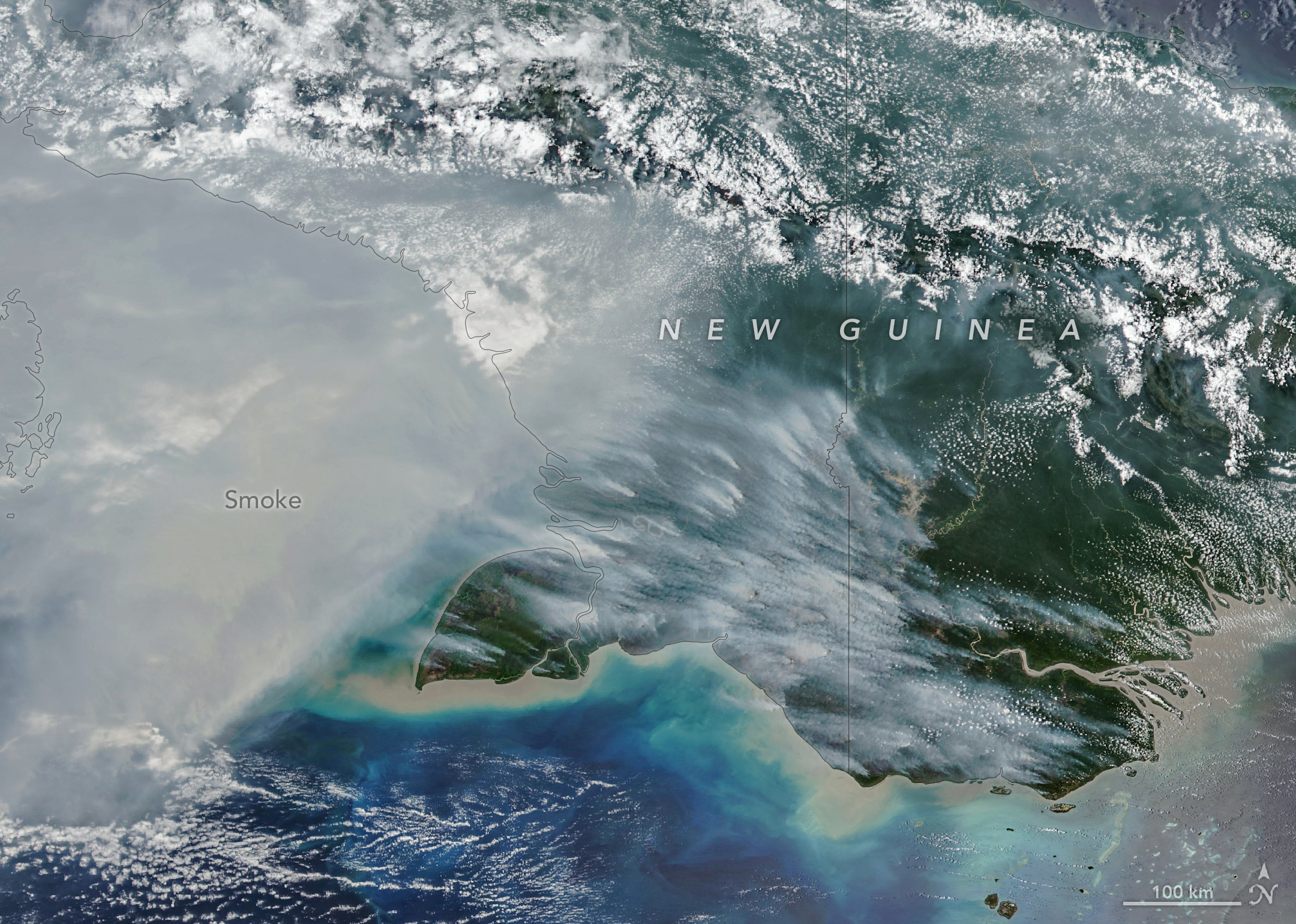
New Guinea, the world’s second-largest island, harbors an extraordinary variety of plant life across more than a dozen distinct ecoregions, including seasonally dry savannas, tropical rainforests, and lowland swamp forests. But in September and October 2026, as drought gripped New Guinea (sometimes called Papua) amid a strong El Niño, fires scorched the island and smoke shrouded large swaths of it for weeks.
The VIIRS (Visible Infrared Imaging Radiometer Suite) on the NOAA-20 satellite captured this image of thick smoke streaming from the southern part of the island on October 11, 2026. In recent weeks, soaring levels of air pollution delayed and canceled flights, closed schools, and prompted officials in some areas to urge children and older people to wear masks.
“Sometimes smoke that has drifted into the convection of nearby thunderstorms will get washed out or lofted up into the upper troposphere, but a lot of smoke stays near the surface and causes air quality problems,” said Robert Field, an associate research scientist at NASA’s Goddard Institute for Space Studies and Columbia University. “It’s a horrible situation.”
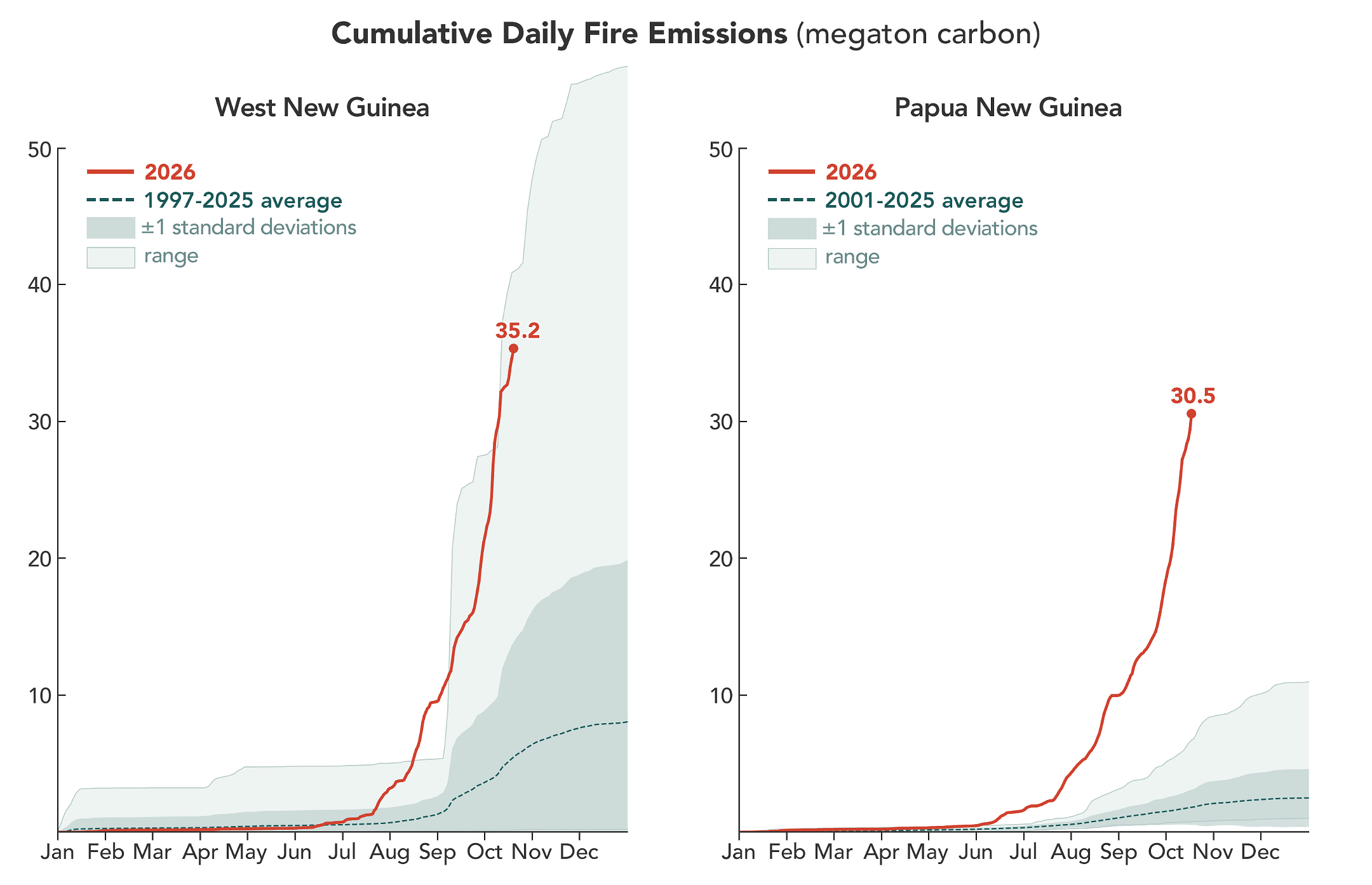
According to the Global Fire Emissions Database (GFED), a fire emissions monitoring system, fires in Papua New Guinea, on the eastern half of the island, had released nearly 32 megatons of carbon by October 17, more than any other year on record at that point in the year (charts above). “Emissions are already much higher than the 2015 total for the year, and it’s very likely that this will become the highest year on record for Papua New Guinea, even surpassing 1997,” said Guido van der Werf, a fire scientist at Wageningen University & Research.
On the Indonesian side, sometimes called West New Guinea or Indonesian Papua, carbon emissions exceeded 35 megatons, the third highest after 2015 and 1997, other El Niño years with severe fires. Van der Werf led the development of GFED, a satellite-driven modeling framework that uses a mix of remote sensing, vegetation characteristics, and other information to estimate the extent of vegetation fires and the emissions over nearly three decades.
In this normally wet part of the world, people ignite the vast majority of fires, researchers say. Crop fires, pasture maintenance, deforestation and land clearing, and hunting are all common reasons people burn in New Guinea. In dry conditions, managed fires sometimes spread and burn uncontrolled as wildfires, particularly in the drier, southernmost parts of the island.
“We’re seeing an exceptionally high level of fire activity in Papua New Guinea and Eastern Indonesia, particularly Indonesian Papua and Kalimantan, this year compared with Sumatra and other parts of Western Indonesia,” said Yang Chen, an associate researcher at the University of California, Irvine. “Papua has emerged as Indonesia’s new deforestation frontier.”
Over the past two decades, land in Indonesian Papua has been cleared for industrial oil palm and pulpwood plantations, shifting small-scale cultivation, urban expansion, and mining. According to Global Forest Watch, the region lost 27,000 hectares of primary forest in 2025, nearly double the 2024 total and the most since 2017.
Sumatra’s fires are relatively low compared to other drought years partly because many areas are already developed. “Areas with large oil palm, sugarcane, or pulpwood plantations also often have their own private fire brigades to protect their assets,” said Field. “It’s in unmanaged areas or primary forest edges where we’re generally seeing the most fire.”
Researchers expect the fires to continue until the heavy rains of the wet season arrive in the southern part of New Guinea, typically in early November.
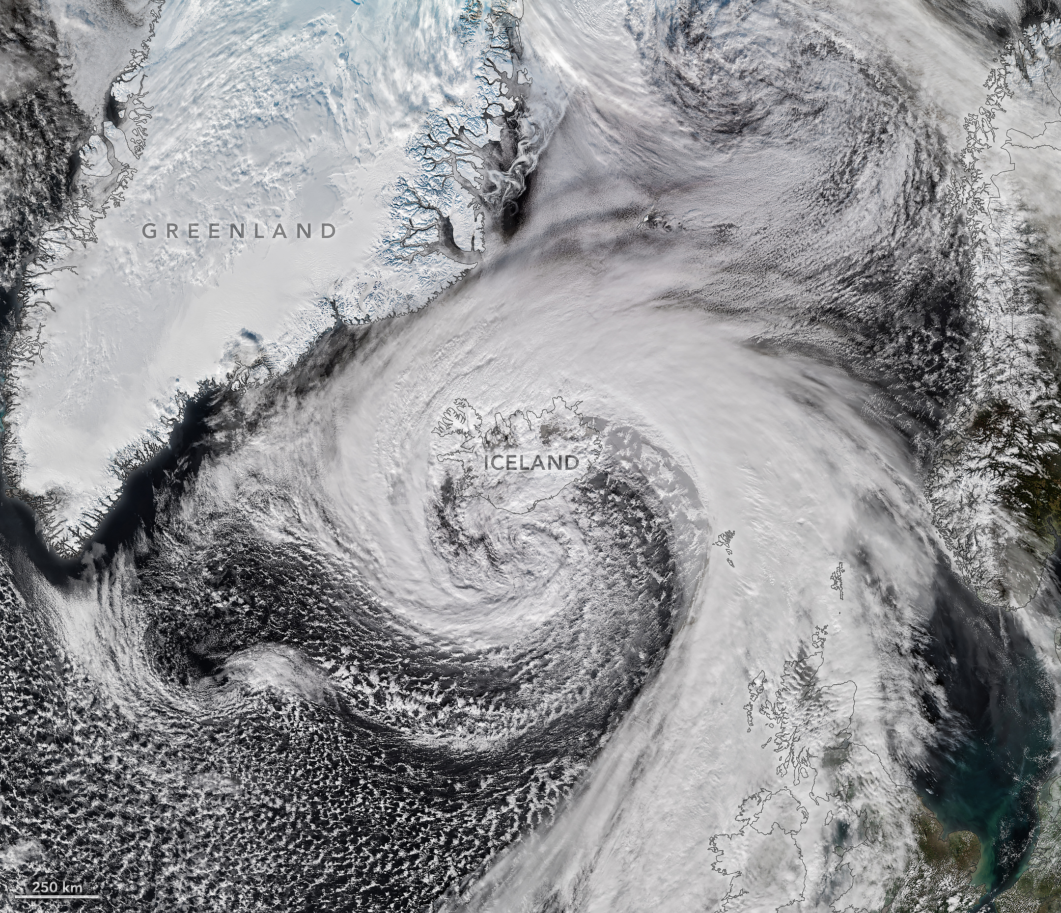
Hurricane Isaias—the only Atlantic hurricane to date in 2026—made landfall in Florida as a Category 2 storm on October 9. After delivering a rainy, windy blow to the U.S. Gulf Coast and drenching much of the Eastern Seaboard, the weather system had more in store.
Riding the jet stream east over the North Atlantic, Isaias’s remnants developed into a powerful storm known as an extratropical cyclone. These low-pressure systems often feature asymmetrical, comma-shaped cloud patterns and can strike with hurricane-force winds, rain, and blizzard-like conditions.
The VIIRS (Visible Infrared Imaging Radiometer Suite) on the NOAA-21 satellite captured this image of the extratropical cyclone brushing past Iceland on the afternoon of October 14. During its journey, the system’s air pressure plummeted by more than 50 hectopascals over a 24-hour period, according to reports—approximately double the criteria for explosive cyclogenesis, or bombogenesis. Some meteorologists believe the storm may have set a new October low for barometric pressure in Iceland, after correcting for altitude, likely breaking a record that has stood since 1963.
The cyclone lashed Iceland with high winds as it grazed the coast. A gust of 205 kilometers (128 miles) per hour was recorded near Eyjafjallajökull volcano in the country’s south, while a small island just offshore saw sustained winds of 150 kilometers (93 miles) per hour. Damaging winds extended into northern parts of the country, where residents also braced for sleet and snow. Farther across the Atlantic, northwestern Scotland received gusts up to 90 kilometers (55 miles) per hour on October 14, according to news reports, resulting in cancellations on several ferry routes.
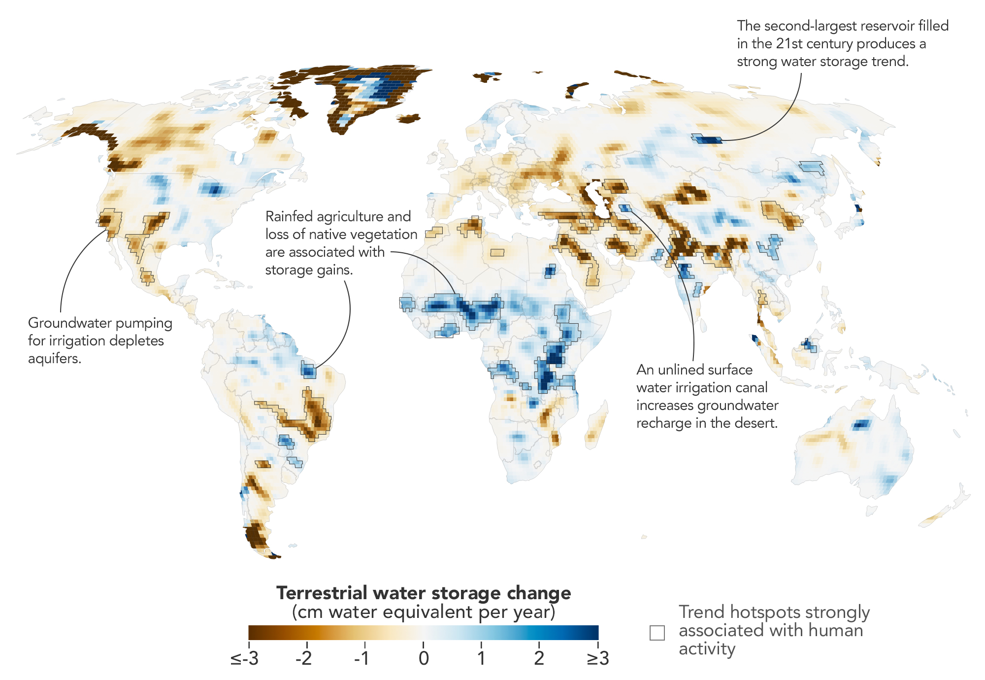
Measurements from NASA’s GRACE (Gravity Recovery and Climate Experiment) and GRACE-FO (GRACE Follow-On) missions reveal trends in terrestrial water storage from April 2002 to November 2025. Areas outlined in black indicate where trends showed strong associations with human activities. Trends are depicted in terms of average annual change in equivalent water depth.
NASA Earth Observatory/Michala Garrison, based on data from O’Neill, M.M., et al.
Humans are exerting increasing influence over how water moves through lakes, rivers, soil, and the subsurface, and a new NASA study shows where those effects are greatest. Using more than two decades of satellite measurements of subtle changes in Earth’s gravity, the researchers sharpened the picture of how—and why—terrestrial water storage has changed.
This map encapsulates their findings, depicting changes in terrestrial water storage from April 2002 to November 2025. Beyond the influence of climate variability, the scientists identified 40 regions where the changes also aligned with human activities such as irrigation, reservoir impoundment, and land-use change. These activities were significantly related to terrestrial water storage trends on every nonpolar continent except Australia.
In some areas, the effects of human activities were especially strong. “In four continental regions, an anthropogenic variable showed a stronger relationship with the storage trends than any climate variable did,” said Mary Michael O’Neill, a hydrologist at NASA’s Goddard Space Flight Center and lead author of the study.
They include well-known spots such as California’s Central Valley and northern India, where farmers’ heavy reliance on groundwater has drawn down storage—in India’s case, faster than earlier estimates suggested. Elsewhere, some types of farming and water management appear to have done the opposite.
Gravity as a Water Gauge
The data behind the map come from the GRACE (Gravity Recovery and Climate Experiment) and GRACE-FO (GRACE Follow-On) missions, each of which consists of two satellites that fly in tandem. As the lead satellite passes over an area with greater mass, the slight change in gravity tugs at it, and instruments aboard the satellites measure the change in distance between them. Since water and ice are heavy and shift around regularly, scientists can use GRACE data to infer gains and losses.
The satellites’ data are typically processed into monthly maps that show broad patterns of water storage. But over more than 20 years, the satellites have passed over most of the planet many times. By combining all of those passes, the researchers could map long-term water trends with five to 10 times more spatial detail than previous analyses. The tradeoff was a loss of temporal detail. They then applied statistical techniques to weigh the importance of various anthropogenic and climatic factors in the storage trends and to pinpoint where human activities may have contributed.
The improved spatial resolution uncovered some human impacts that had not been previously detected, said Matthew Rodell, deputy director of Earth Sciences for Hydrosphere, Biosphere, and Geophysics at Goddard and one of the study’s authors. The analysis also showed that some known trends were stronger than previously realized.
Where the Water Went
Across several continents, groundwater-irrigated farmland was strongly associated with declines in terrestrial water storage. In North America, these declines appeared in California’s Central Valley, the southern High Plains of the U.S., and Chihuahua, Mexico, where long-term droughts have increased farmers’ reliance on groundwater. Groundwater pumping also drove declines in northern India, where the refined analysis showed a steeper downward trend than previously realized. Consistent with previous findings, retreating Himalayan glaciers accounted for only 15 percent of the decline there.
Other types of agriculture had a different relationship with water storage trends. In parts of sub-Saharan Africa, for example, some increases occurred where rainfed cropland has expanded. There, swaths of native savanna were replaced by millet cultivation throughout the study period, and water tables rose despite below-average precipitation. A similar pattern emerged in northern Brazil’s Maranhão state, where soybean fields have replaced forests and shrublands. The resulting water storage trend might be explained in part by the efficient water use of cereal and legume plants and by Indigenous practices that help direct water into shallow aquifers, the researchers said.
Water storage and diversion projects also came into focus on the new map. Hundreds of large reservoirs were filled during the study period, the authors note, but the coarse spatial resolution of gravity measurements previously made them difficult to track. In the new analysis, the Boguchany Reservoir on Russia’s Angara River, the second-largest reservoir filled in the 21st century, produced the strongest water storage trend in nonpolar northern Asia.
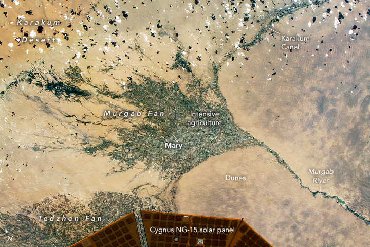
A segment of the Karakum Canal, which diverts river water to irrigate cropland in the desert, is visible as a linear, vegetated feature in this photo, taken by an astronaut aboard the International Space Station on June 13, 2021.
The map also resolves smaller reservoirs and other hydrologic engineering projects. The Karakum Desert in Turkmenistan registered water storage gains stemming from the long, largely unlined Karakum Canal running through it. The canal diverts river water to support desert agriculture, but enough seeps into the ground during its journey to alter the water picture in the desert. The map’s finer resolution allows for better monitoring of such hydrologic changes in remote areas where other measurement options may be limited.
Moving forward, O’Neill wants to capture how dams, diversions, irrigation, and other controls on Earth’s water affect storage downstream, and to disentangle the influence of local and non-local activities. “I’d also like to recover more of the temporal picture,” she said. One way to do that is by combining the higher-resolution data with standard monthly products or by applying the recent technique over shorter timeframes. “This could help track how localized trends evolve in response to specific events like droughts or policy changes.”
NASA Earth Observatory map by Michala Garrison, using data from O’Neill, M.M., et al. (2026).Astronaut photographISS065-E-111045 was acquired on June 13, 2021, with a Nikon D5 digital camera using a focal length of 1,150 millimeters. It is provided by the ISS Crew Earth Observations Facility and the Earth Science and Remote Sensing Unit at NASA Johnson Space Center. The image was taken by a member of the Expedition 65 crew. The image has been cropped and enhanced to improve contrast, and lens artifacts have been removed. The International Space Station Program supports the laboratory as part of the ISS National Lab to help astronauts take pictures of Earth that will be of the greatest value to scientists and the public, and to make those images freely available on the internet. Additional images taken by astronauts and cosmonauts can be viewed at the NASA/JSC Gateway to Astronaut Photography of Earth. Story by Lindsey Doermann.
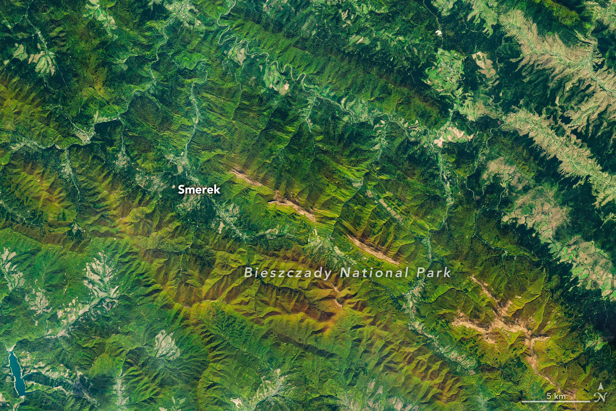
As the air grows cooler and days shorter, brown bears prowl the Carpathian Mountains of southern Poland with the goal of fattening up ahead of winter hibernation. In a more conspicuous sign of autumn, beech and other deciduous trees blanketing the hillsides start to sport reds and golds. The seasonal transformation was underway in southeast Poland’s Bieszczady National Park on October 8, 2026, when the OLI (Operational Land Imager) on the NASA-USGS Landsat 9 satellite captured this image.
European beech (Fagus sylvatica) dominates the area’s forests, with other species such as sycamore maple (Acer pseudoplatanus) also contributing to vibrant color in the fall. Dropping air temperatures and waning daylight cause these trees to curtail the production of chlorophyll, the molecule that plants use to synthesize food. Without it, the leaves’ green pigments fade, allowing the yellows and reds of other pigments to show through.
A descendent of ice-age survivors, the European beech has persisted across millennia in a range of climates. After the glaciers retreated, beech forests spread northward across the European continent from isolated refugia in the Carpathians, Alps, and other mountain ranges, and played a crucial role in reforesting the previously ice-covered land. Portions of Bieszczady National Park are included within UNESCO’s network of ancient and primeval beech forests spanning 18 countries.
Expansive as their footprint across Europe may be, beech forests reach only so high in elevation—about 1,000 to 1,260 meters (3,300 to 4,100 feet)—in this area. Above that is the realm of the polonina, a Slavic term for subalpine meadow, consisting of open grasslands and shrubby thickets of rowan (mountain ash), willows, and green alder. Patches of polonina stretch across ridge tops to the east-southeast of Smerek and appear tan, having lost their summer greenness.
The Bieszczady Mountains are renowned not only for forests and mountain meadows but also for charismatic wildlife. European bison, once extinct in the wild, were reintroduced to the area in the 1960s and now roam the hills by the hundreds, according to recent surveys. Additionally, populations of brown bears and Eurasian lynx find refuge and ample food sources in the forests.
NASA Earth Observatory image by Michala Garrison, using Landsat data from the U.S. Geological Survey. Story by Lindsey Doermann.
Nighttime lights along the Florida Panhandle coast in August 2026, brightest in Pensacola and Destin and along the road between them.
NASA Earth Observatory / Lauren Dauphin
Nighttime lights along the Florida Panhandle coast on October 11, 2026, after Hurricane Isaias, with fewer and dimmer lights in Pensacola and Destin and gaps along the road between them.
NASA Earth Observatory / Lauren Dauphin
August 2026 Composite
October 11, 2026
Lights around Pensacola, Florida, and along the U.S. Route 98 corridor toward Destin appear sharply reduced on October 11, 2026 (right), compared with typical conditions in August 2026 (left), suggesting widespread power outages after Hurricane Isaias. Images are from NASA’s Black Marble HD product.
After a quiet start to the 2026 Atlantic hurricane season, Isaias became the season’s first hurricane on October 8 as it tracked toward the U.S. Gulf Coast. The storm brought heavy rain and flash flooding to parts of the Southeast, including Alabama and the Florida Panhandle, and winds that toppled trees and downed power lines, leaving many people in the dark.
Isaias made landfall near Destin, Florida, on the evening of October 9 as a Category 2 hurricane with maximum sustained winds of 105 miles (170 kilometers) per hour. Gusts topped 100 miles per hour along a corridor west of the storm’s center, according to the National Weather Service, with preliminary reports showing a 117-mile-per-hour gust in Oriole Beach and a 102-mile-per-hour gust at Pensacola City Hall.
These areas of high winds overlapped a broader area west of the storm’s eye where satellite images showed substantial decreases in nighttime lights. The image pair above shows nighttime lights before and after the storm. The left image is a composite of August 2026 data representing typical conditions, and the right image shows lights on October 11, after most of the storm’s clouds had cleared.
The data depicted in the images, provided by Ranjay Shrestha of NASA’s Black Marble science team, come from the Black Marble HD product. The product uses data from the VIIRS (Visible Infrared Imaging Radiometer Suite) on the NOAA-20 satellite, which has a day-night band that detects light emitted and reflected at night. The team processed the data to account for changes in the landscape, the atmosphere, and phase of the Moon, and to filter out stray light that does not come from electric lights. Dark gray, hash-marked areas show where clouds prevented VIIRS from collecting data. The nighttime lights are shown over a base map from the Landsat 9 satellite.
“Standard Black Marble nighttime lights imagery, available through NASA Worldview, provides a broad picture of the storm’s immediate impacts,” Shrestha said. “Black Marble HD takes this a step further by allowing us to visualize these changes at a much finer spatial scale.”
At these finer scales, the images reveal lights decreasing sharply around parts of Pensacola, Florida, and along the U.S. Route 98 corridor toward Destin, suggesting widespread power disruptions. Shrestha also pointed out pockets where lights persisted, including Pensacola International Airport, Pensacola Christian College, and parts of downtown Pensacola. “These patterns could reflect backup power systems, differences in electrical infrastructure, or areas that maintained electricity during the storm, although the imagery alone cannot confirm the underlying reasons,” he said.
October 11, 2026
October 12, 2026
Nighttime lights along the Florida Panhandle coast on October 11, 2026, after Hurricane Isaias, with fewer and dimmer lights in Pensacola and Destin and gaps along the road between them.
NASA Earth Observatory / Lauren Dauphin
The same area on October 12, 2026, with lights in Pensacola and Destin and along the road between them closer to pre-storm levels.
NASA Earth Observatory / Lauren Dauphin
October 11, 2026
October 12, 2026
Widespread outages darken the region around Pensacola, Florida, and along the U.S. Route 98 corridor toward Destin on October 11, 2026 (left). By October 12 (right), lights have returned to some affected areas. Images are from NASA’s Black Marble HD product.
Black Marble HD images also reveal the pace and spatial patterns of recovery. The image pair above compares the same October 11 view (left) with one from October 12 (right), when lights had begun to return to some affected areas. By October 14, lighting patterns looked similar to pre-storm conditions.
“Understanding where recovery is progressing and where disruptions persist can help emergency responders and decision makers identify areas that may require additional attention, prioritize resources, and assess the effectiveness of restoration efforts,” Shrestha said.
Black Marble data complement ground-based outage reports rather than replace them, offering a more comprehensive view of disasters’ impacts and recovery. “Ultimately, this is where the value of Black Marble lies: turning nighttime Earth observations into actionable insights that support informed decisions and help bridge the gap between Earth science and action,” Shrestha said.
The NASA Disasters Program, in coordination with FEMA and the USGS Coastal Storms Team, is supporting the Alabama Red Cross and the Alabama Emergency Management Agency’s response to Hurricane Isaias. The team will be posting maps and data products on its open-access mapping portal as new information becomes available.
NASA Earth Observatory images by Lauren Dauphin, using Black Marble HD data courtesy of Ranjay Shrestha/NASA’s Goddard Space Flight Center and Landsat data from the U.S. Geological Survey. Story by Kathryn Hansen.
Unlike a tornado or thunderstorm that can deliver destruction in minutes, El Niño exerts its influence over many months. This year, a drought accompanying El Niño has left the Amazon rainforest primed to burn, and scientists say the region has entered the early stages of what they think will be a long and severe fire season.
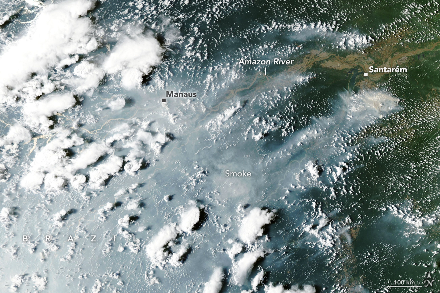
Starting in September 2026, satellites detected sharp increases in fire activity and smoke emissions in the central and eastern Amazon, visible in fire and emissions monitoring platforms including NASA’s Fire Information for Resource Management System (FIRMS), the Global Fire Emissions Database (GFED), and NASA Worldview. The region with elevated fire activity stretches from forests surrounding the commercial and transportation centers of Manaus and Santarém to the mouth of the Amazon River.
When the MODIS (Moderate Resolution Imaging Spectroradiometer) on NASA’s Aqua satellite captured this image of smoke streaming from fires on both sides of the Amazon River on October 12, 2026, heavy smoke socked in Manaus, the capital of the Brazilian state of Amazonas. That day, city officials reported extremely poor air quality, with fine particulate matter (PM2.5) values above 135 micrograms per cubic meter, the second-worst rating on a regional air quality index. The pall disrupted daily life in a city of more than 2 million people. Schools closed, and citywide events and children’s sports leagues were canceled as officials warned of hazardous air quality, according to news reports.
The burning around Santarém and Manaus is part of a “cascade” of fire in the tropics that accompanies the disrupted rainfall patterns of an El Niño, said Douglas Morton, an Earth system scientist based at NASA’s Goddard Space Flight Center. The pattern begins along the equator with drought and peat fires in Indonesia, followed by elevated fire activity in this part of the Amazon. Morton and colleagues from the University of California, Irvine; Vrije Universiteit Amsterdam; and the University of Maryland detailed the pattern in a 2017 study following the destructive fire season that accompanied the 2015–2016 El Niño. They also saw the pattern play out in 2023.
A swell of fire in the tropics riding the 2026 El Niño has followed the pattern. Drought, fire, and smoke have smothered parts of Indonesia since August, with hundreds of homes razed in October and thick smoke blanketing whole islands most days. “Now, in the Amazon, we’re seeing the second domino in the cascade fall,” Morton said, referring to the uptick in fires that has begun in Pará and Amazonas.
Morton and his colleagues expect the next wave of fire to hit farther north in November and December in the Brazilian states of Roraima, northern Pará, and Amapá, as well as parts of Venezuela, Guyana, and Suriname. Finally, around August and September 2027, he said, drought and fire risk will peak in the southern Amazon regions of Brazil and Paraguay.
“It’s so striking—and frustrating—that this is happening all over again,” said Morton, adding that many of the same forests that burned during the El Niño events in 2023 and 2015 are burning again. Forest fires in these rainforests are known to cause especially serious ecological damage because most species are not adapted to fire. It’s likely that some of the forest fires will burn even more intensely this time because the earlier fires partially charred trees, degrading the forest and making what remained more susceptible to burning, he added.
Morton expects the fires around Santarém and Manaus to continue burning until the rainy season arrives in December 2026 or January 2027. For the regions to the north and south, there is still time to prepare. “Given the intensity of this El Niño, this really is the year for people to avoid burning at all costs,” Morton said.
It’s so wet in the Brazilian Amazon that lightning ignites less than 1 percent of fires, so the vast majority of fires currently burning there were started by people, Morton said. But this year’s drought, worsened by El Niño, has been intense. Brazil’s National Institute of Meteorology reported that Manaus rainfall levels were 95 percent less than normal in August and 60 percent less than normal in September.
The large fires in this region began as management fires—clearing shrubs from pastures or crops from fields, for instance—but have escaped and are now burning freely through the parched understory of the rainforest, he added. Analysis of satellite observations indicates there are 50 to 70 uncontrolled fires burning in the Santarém region alone, said Shane Coffield, a University of Maryland assistant research scientist at NASA Goddard.
As part of a NASA Earth Action project, Coffield is mining fire observations from VIIRS (Visible Infrared Imaging Radiometer Suite) to identify fires that didn’t meet the threshold for inclusion in official data products distributed by FIRMS. He plans to share the locations of these “candidate fires” with scientists at MapBiomas, a multi-institutional network comprising universities, NGOs, and technology companies that maps fires and land-use change in the Amazon.
“For the area around Santarém, we’ve identified about 40 percent more fires than you’ll see in active fire counts from FIRMS,” said Coffield. Satellites often miss fires in circumstances like this due to dense smoke, clouds, and tree canopy cover, which can block the sensors from detecting the infrared signal of fires—especially lower-intensity fires spreading along the forest understory. “On some of the smokiest days, we have very few detections from MODIS and VIIRS, and we know that isn’t right.”
NASA Earth Observatory images by Lauren Dauphin, using MODIS data from NASA EOSDIS LANCE and GIBS/Worldview. Story by Adam Voiland.
Astronomers have used NASA’s Chandra X-ray Observatory to break down the cause of a remarkable formation of radio waves they have nicknamed the “Treble Clef” because its distinct shape strongly resembles the musical symbol.
The researchers discovered the Treble Clef is likely caused by an outburst from a supermassive black hole, followed by a collision of two galaxy clusters. A paper describing the findings, led by Andrea Botteon of the National Institute for Astrophysics, or INAF, in Italy, published Wednesday in the Astronomy & Astrophysics journal.
An explanation for the Treble Clef has been particularly difficult to find because the formation lies almost directly behind the plane of the Milky Way, meaning that stars, gas, and dust from our home galaxy largely block the view from Earth. However, by using telescopes that can peer through the intervening material, a team of researchers was able to identify what is responsible for this uncommon structure.
NASA’s Chandra and the German Extended RÖntgen Survey with an Imaging Telescope Array (eROSITA) X-ray telescope found diffuse, hot gas at the location of the Treble Clef, showing that a galaxy cluster hosts the object. The researchers also determined the galaxy cluster is, in fact, two clusters in the process of merging. Galaxy clusters are some of the largest structures in the universe, containing hundreds of individual galaxies and huge reservoirs of superheated gas.
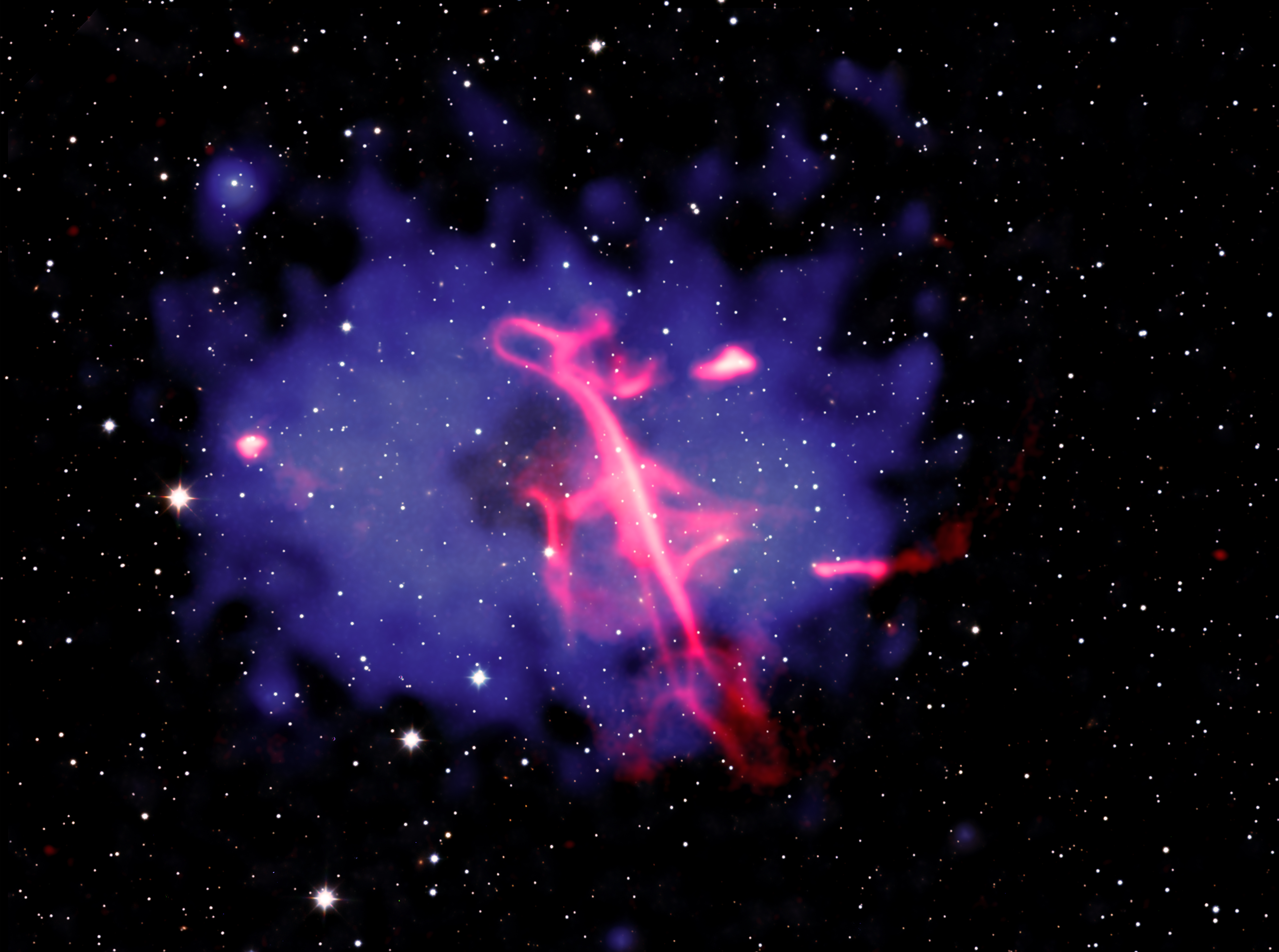
This new composite image of the Treble Clef and its cluster shows the multimillion-degree gas detected in X-rays by Chandra and eROSITA in blue, with some of the Chandra data derived from a special technique the authors used to highlight important features in the Chandra data. Radio data shown in red from the LOw Frequency ARray (LOFAR), a large network of radio telescopes in Europe reveals the doppelganger of the musical notation. The final piece of the combined image comes from infrared data obtained by the United Kingdom Infrared Telescope, appearing mostly white.
The authors concluded that the Treble Clef likely formed in a two-stage process. First, an earlier outburst from a supermassive black hole in the galaxy cluster’s center drove clouds of charged particles and magnetic fields away at close to the speed of light. This led to a type of cosmic crescendo and initially produced bright radio waves that later faded as the particles lost energy. Next, the collision between the two clusters compressed or reenergized the cloud, which became brighter again in radio waves. Shock waves — similar to the sonic booms from supersonic jets — from the collision may have played a role in this reenergizing process.
To reveal evidence for the cluster collision in the Chandra data, the authors used a special technique that examined how much the cluster’s hot gas deviates from a symmetrical shape. Most of the hot gas is symmetrical and shaped approximately like an oval. The authors removed this symmetrical oval shape from the original X-ray image. The remaining X-ray emission in the residual image shows t is brightest on the left and right, and faintest in the center. The new composite image combines both the original X-ray and the residual X-ray images.
The brighter X-rays in the residual image, toward the left and right of the cluster’s center, imply that the collision between the two clusters likely occurred along the left-right direction as seen in the image. The researchers think the direct collision between the two clusters occurred a few hundred million years ago, and the clusters are now moving away from each other.
The resemblance to a treble clef is a case of pareidolia, the phenomenon when people see familiar shapes in random data, since there is no scientific connection to the musical notation.
NASA’s Marshall Space Flight Center in Huntsville, Alabama, manages the Chandra program. The Smithsonian Astrophysical Observatory’s Chandra X-ray Center controls science operations from Cambridge, Massachusetts, and flight operations from Burlington, Massachusetts.
This release features a composite image of a remarkable radio wave formation that strongly resembles a treble clef musical symbol, hovering in the midst of two colliding galaxy clusters.
Here, galaxies in the galaxy clusters, plus foreground and background stars and galaxies, blanket the image with specks of light set against the blackness of space. At the center of the frame is a large, oval, blue-purple cloud with ragged edges. This is a multimillion-degree gas cloud in the two clusters detected in X-rays by Chandra and eROSITA, the Extended RÖntgen Survey with an Imaging Telescope Array.
In the middle of the purple field, tilting slightly to our left, is what appears to be a giant treble clef, loosely drawn with a neon pink marker. Like the musical notation for which it’s named, the formation has a strong vertical stroke with a continuous, fluid line swooping back and forth as it moves from top to bottom.
This radio wave formation appears to be the result of a two-stage process. First, charged particles and magnetic fields were driven from a supermassive black hole, producing bright radio waves. Those waves faded and lost energy over time, before being reenergized and compressed when the two galaxy clusters collided.
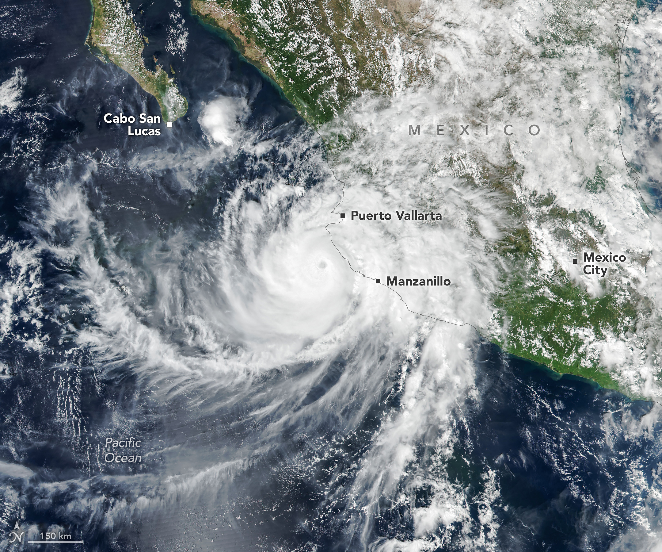
Hurricane Simon churns off Mexico’s Pacific coast in this image acquired with the VIIRS (Visible Infrared Imaging Radiometer Suite) on the Suomi NPP satellite on October 11, 2026.
NASA Earth Observatory/Michala Garrison
Hurricane Simon, the latest in a long progression of tropical cyclones in the Eastern Pacific this season, passed close to the Mexican coast as a category 4 storm on October 11, 2026. Sustained winds reached 250 kilometers (155 miles) per hour as it crept north-northwest.
Simon’s eye was about 50 kilometers (30 miles) offshore, between Manzanillo and Puerto Vallarta, when the VIIRS (Visible Infrared Imaging Radiometer Suite) on the Suomi NPP satellite acquired this image around 2:30 p.m. local time (20:30 Universal Time) on October 11.
By that time, sustained winds were about 210 kilometers (130 miles) per hour, according to the National Hurricane Center (NHC), and the storm’s inner core was brushing up against the coast. The topography of the Sierra Madre mountains appeared to temper the storm’s intensity somewhat and shrink the size of its wind field, the NHC noted. Still, the major hurricane delivered heavy rain and flooding to coastal areas, including the port city of Manzanillo, and raised the risk of mudslides in mountainous areas, according to news reports.
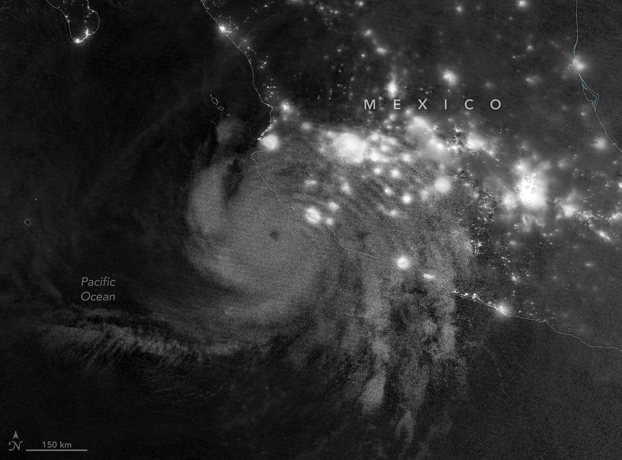
Atmospheric gravity waves generated by Hurricane Simon are visible via mesospheric airglow in this nighttime image acquired with the VIIRS (Visible Infrared Imaging Radiometer Suite) on the NOAA-21 satellite on October 11, 2026.
NASA Earth Observatory/Michala Garrison
In the early morning hours of October 11, satellites captured the storm’s effects extending into the upper atmosphere. This nighttime image (above), acquired with VIIRS on the NOAA-21 satellite, shows atmospheric gravity waves radiating from the hurricane. These ripples form when latent heat released near the tropical cyclone’s eyewall drives strong convection, building tall cumulonimbus clouds with updrafts that can send waves into the stratosphere and mesosphere.
But these waves are not always observable. Winds in the upper atmosphere can dissipate them before they reach the mesosphere, where they show up as ripples in airglow—faint light emitted by gases at those high altitudes. The VIIRS day-night band is sensitive to airglow but also detects reflected moonlight, which can wash it out. On the night this image was acquired, minimal illumination from the Moon helped the airglow stand out.
On the morning of October 13, forecasts of Simon’s intensity and path remained “very low confidence,” as the storm’s evolution continued to defy meteorologists’ expectations. The system may steer north and enter the Gulf of California before making landfall. Large swells causing dangerous nearshore conditions were expected along portions of the southwestern and west-central coasts of Mexico in the coming days.
Editor’s Note: Today’s story is the answer to the October Puzzler.
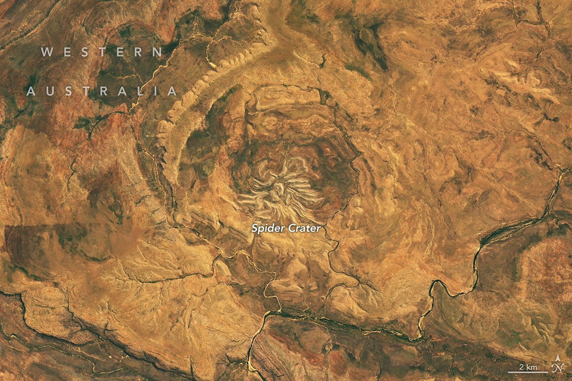
From above, the mere appearance of a curious geologic feature in Western Australia is enough to cause a fright. The aptly named Spider Crater, the product of a meteorite impact followed by hundreds of millions of years of erosion, sprawls across the landscape in the country’s Kimberley region.
The OLI (Operational Land Imager) on the NASA-USGS Landsat 9 satellite captured this image of the crater on September 20, 2026. The full impact structure has an oval shape measuring about 13 kilometers by 11 kilometers (8 miles by 7 miles), with the spiderlike central portion measuring about 4 kilometers (2.5 miles) across.
Geologists believe the unusual arachnoid pattern is the remnant of a central uplift, the raised portion of the crater floor that formed in the rebound of the initial impact shock. The light-colored “legs” are sandstone ridges that have endured while other rock layers in the impact zone have eroded away.
For decades after the feature’s discovery, scientists struggled to weave a tale about its formation. Some proposed it had a volcanic past. But with some legwork in the field, geologists identified telltale signs of a past impact: fan-shaped fractures called shatter cones. These fractures form only when intense shock waves travel through rock, and they are ubiquitous in Spider Crater’s central dome.
Scientists have subsequently performed lab analyses of shocked quartz and zircon crystals from the sandstone, which can help them reconstruct the angle of the meteorite’s impact. The date of the impact is uncertain, but estimates based on rocks in the region place it between about 900 million and 600 million years ago—making Spider Crater a creature of the late Precambrian.
NASA Earth Observatory image by Michala Garrison, using Landsat data from the U.S. Geological Survey. Story by Lindsey Doermann.
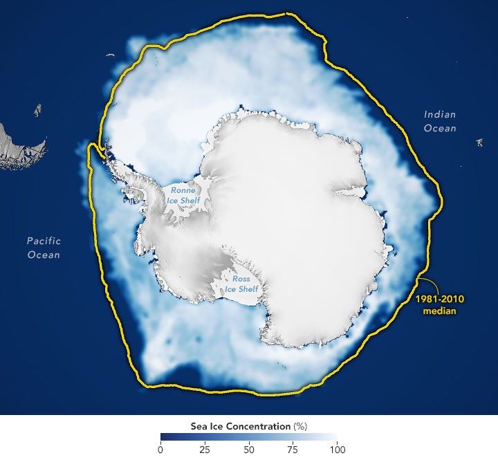
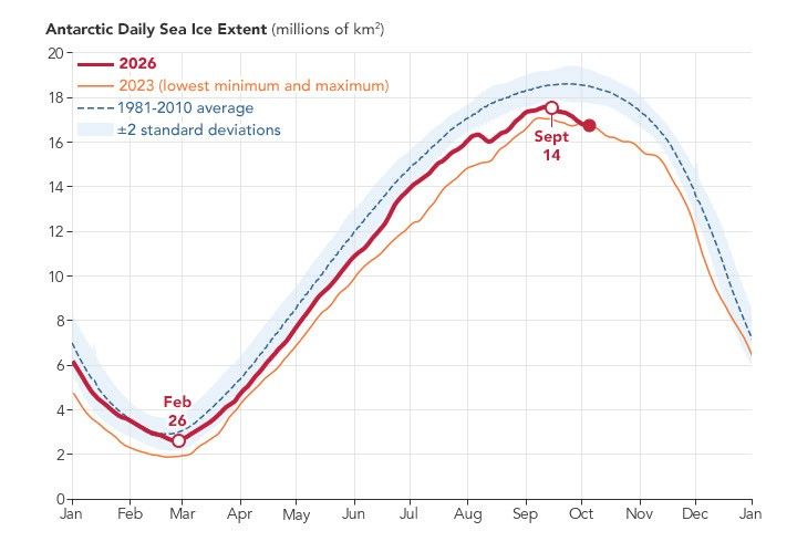
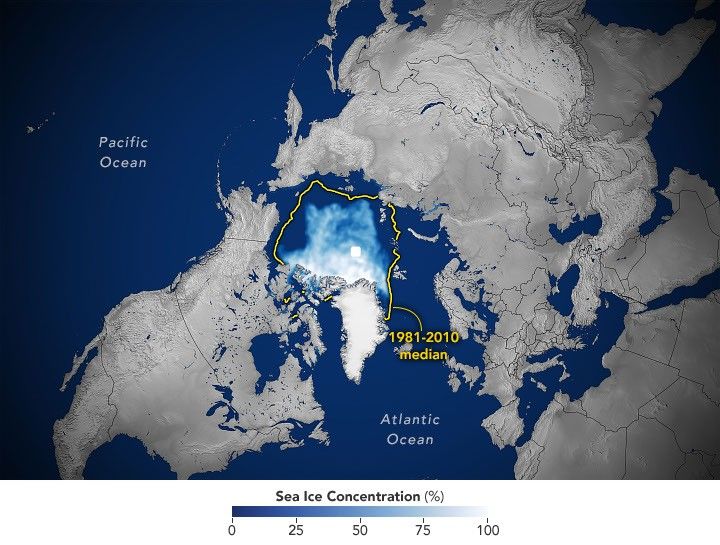
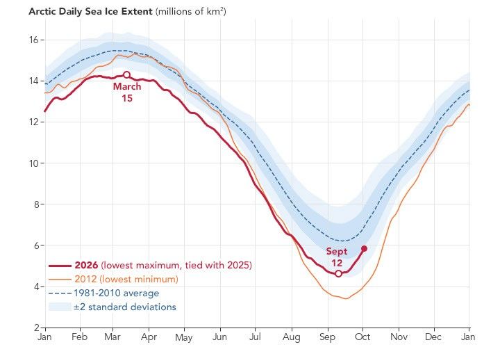
Antarctic sea ice reached its annual maximum extent on September 14, 2026—the third-lowest maximum in the satellite record.
NASA Earth Observatory/Michala Garrison
This story is an update to the Antarctic sea ice feature in our World of Change series tracking long-term change on Earth’s surface through satellite imagery.
Unlike the Arctic—an ocean basin surrounded by land—the Antarctic is a large continent surrounded by an ocean. Because of this geography, sea ice has more room to expand during the winter. However, that ice also stretches into warmer latitudes, leading to more melting in the summer. Antarctic sea ice usually peaks in September, around the end of the Southern Hemisphere’s winter, and retreats to a minimum in February.
According to NASA and the National Snow and Ice Data Center (NSIDC), Antarctic sea ice in 2026 likely reached its annual maximum extent on September 14 (above). On that date, the ice covered an estimated 17.59 million square kilometers (6.79 million square miles), making it the third-lowest maximum on record.
The maps below show the average concentration of Antarctic sea ice for the month of September (left) and the following February (right) from 1990 to 2026. Opaque white areas indicate the highest concentrations, and dark blue areas are open water. The images include only areas where ice concentration was at least 15 percent, a threshold scientists commonly use to count an area as ice-covered in satellite data. Scientists refer to the total area of these regions as the “sea ice extent.”
1990-1991
1991-1992
1992-1993
1993-1994
1994-1995
1995-1996
1996-1997
1997-1998
1998-1999
1999-2000
2000-2001
2001-2002
2002-2003
2003-2004
2004-2005
2005-2006
2006-2007
2007-2008
2008-2009
2009-2010
2010-2011
2011-2012
2012-2013
2013-2014
2014-2015
2015-2016
2016-2017
2017-2018
2018-2019
2019-2020
2020-2021
2021-2022
2022-2023
2023-2024
2024-2025
2025-2026
From Record Highs to Record Lows
From 1979 until 2014, total Antarctic sea ice increased by about 1 percent per decade. Whether the increase was a sign of meaningful change is uncertain because ice extents vary considerably from year to year around Antarctica. For three consecutive years, from 2012 to 2014, satellites observed new record highs for winter sea ice extent. These highs occurred while Arctic ice was in steep decline.
The climb came to an end in 2015, and significant decreases in sea ice around Antarctica started to occur in 2016. There have since been years with small rebounds, but overall, Antarctic sea ice coverage has largely remained lower than normal. Both the record low minimum and record low maximum occurred in 2023. Scientists will continue to observe the area each year to find out if the decline is part of a long-term change or a statistical fluctuation.
Seeing Through the Clouds
To determine sea ice extent, scientists rely on satellites with passive microwave sensors that measure the microwave energy Earth naturally emits. Sea ice emits more of this energy than open water, so it stands out in microwave images. Because microwaves pass through clouds, the satellites can observe sea ice regularly, regardless of weather.
A narrow river (dark blue) meanders across vegetated land (bright green) in a false-color satellite image. Small geometric ponds or waterlogged fields appear on the left side of the scene.
NASA Earth Observatory / Lauren Dauphin
In a false-color satellite image of the same area, floodwaters (dark blue) flank a meandering river and cover a large swath of agricultural or aquacultural land primarily on the left side of the scene.
NASA Earth Observatory / Lauren Dauphin
October 7, 2025
October 2, 2026
September falls in the heart of the monsoon season in Thailand, where cities and towns are accustomed to the afternoon rains and thunderstorms that frequently roll through. But throughout late September and early October 2026, persistent heavy rains punctuated by intense downpours left low-lying areas across the country in Southeast Asia under sustained flooding.
Prachin Buri province was among the areas where flooding was widespread. The right image above shows land along the Bang Pakong River and nearby agricultural areas and aquaculture facilities inundated on October 2, 2026. The left image shows the same area at the same time of year in 2025. Acquired with NASA-USGS Landsat satellites, the images are false-color to better distinguish water from vegetation, developed land, and other surfaces. The bright red shapes are floating solar arrays.
Some of the flooding likely stemmed from a low-pressure system that stalled over the area for several days in late September. Stoked by moisture and energy from the warm Gulf of Thailand nearby, the system delivered especially intense rains to the region. About 100 kilometers (60 miles) to the west, Bangkok received nearly 300 millimeters (11.8 inches) of rain over a 48-hour period, according to news reports, close to the average monthly rainfall total for September of 344 millimeters (13.5 inches).
Since mid-September, flooding has occurred in 50 provinces across the country, affecting over 4 million people and causing dozens of deaths, according to the International Federation of Red Cross and Red Crescent Societies. Government agencies estimate about 270,000 hectares (670,000 acres) of farmland, including rice fields and fruit orchards, have been damaged.
NASA Earth Observatory images by Lauren Dauphin, using Landsat data from the U.S. Geological Survey. Story by Lindsey Doermann.
A satellite image of farmland around Lubbock, Texas, on September 22, 2025, features a patchwork of green and brown agricultural fields and several playa lakes with varying amounts of water.
NASA Earth Observatory / Lauren Dauphin
A satellite image of the same Lubbock region on September 9, 2026, appears parched, with much less green vegetation and mostly dry lakes.
NASA Earth Observatory / Lauren Dauphin
September 22, 2025
September 9, 2026
Fields were parched and brown, and playa lakes mostly dry, in Lubbock County in September 2026 (right) compared to September 2025 (left) in imagery captured by the OLI (Operational Land Imager) on the NASA/USGS Landsat 8 satellite. NASA Earth Observatory/Lauren Dauphin
For many longtime cotton farmers in the Texas High Plains, the 2026 drought sparked flashbacks to catastrophic harvests of the past. Miserably dry seasons forced farmers in America’s largest cotton-producing region to abandon massive portions of their dryland crop, including 72 percent in 2022 and 66 percent in 2011.
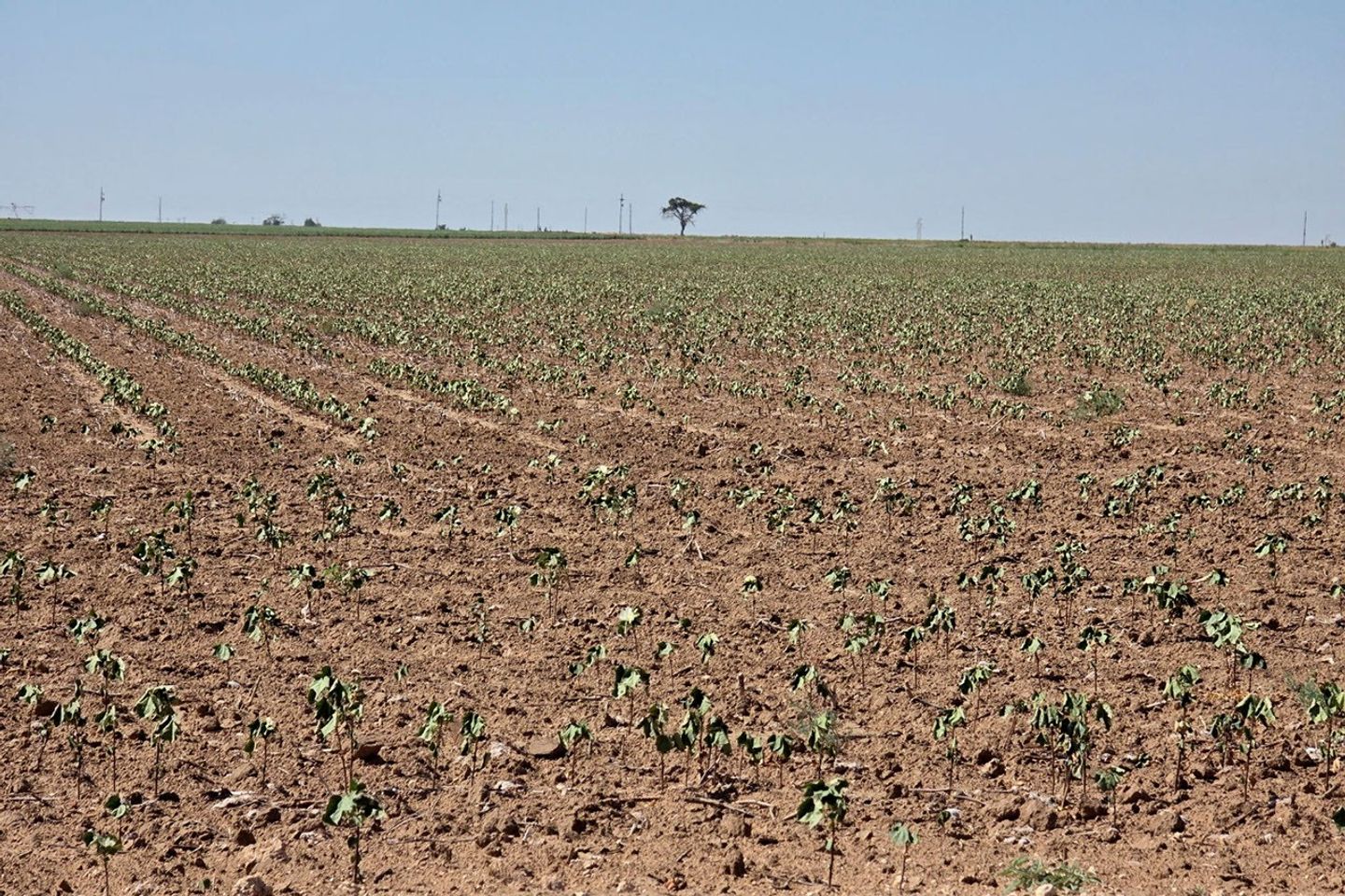
But in some ways, farmers felt the drought in 2026 entered new territory. “This is the first year that we’ve had cotton completely die,” said Lacy Cotter-Vardeman, a farmer based in Lubbock County whose family has worked the land there for several generations. “I was just talking to our insurance people, and they said they’d never seen this before,” she said, adding that roughly 90 percent of her dryland cotton was dead.
Satellite images highlight the scale of the problem in Lubbock and adjacent counties. Brown, parched crops and vacant plots dominated the landscape on September 9, 2026, when the OLI (Operational Land Imager) on Landsat 8 captured the image above (right). In contrast, much greener landscapes prevailed on September 22, 2025 (left), when the sensor captured an image of the same area during a more typical year with a relatively healthy harvest.
Rows of spindly, wilted cotton photographed in one of Cotter-Vardeman’s fields in Slaton, Texas, appear stressed and near death on August 14, 2026.
Lacy Cotter-Vardeman
Subtler signs of the drought are also visible. With groundwater growing scarce in the High Plains aquifer, many farmers in the region have started irrigating just one-half or one-third of their center-pivot fields, explained Tillery Timmons-Sims, an agricultural conservationist who owns land in Brownfield, Texas, and used to grow cotton. In the imagery, these appear as green semicircles and quarter circles.
Note also the many shallow water features known as playa lakes—sometimes called mud holes, buffalo wallows, and lagoons—scattered throughout the image. Some, like Double Lakes and Mound Lake, are fairly large, but most of the more than 19,300 playa lakes in the Texas High Plains are quite small, less than 30 acres.
Many of these ephemeral lakes were dry in September 2026, unlike the previous year. Playa lakes are critical in this water-stressed region because the clay-lined features, if active, collect rainfall and provide pathways for water to seep underground and recharge the aquifer below, the region’s primary source of irrigation water. However, about 80 percent are modified by tilling or buried with sediment, and many no longer function that way.
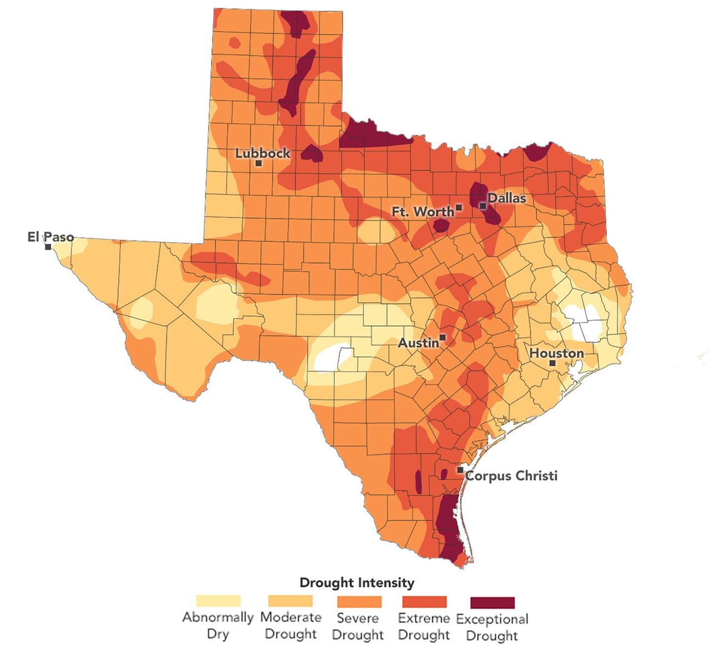
Drought remained severe across many parts of the Texas High Plains in October 2026 despite some rain falling in recent weeks. The data depicted in the map are produced by the U.S. Drought Monitor, a partnership between the National Drought Mitigation Center at the University of Nebraska-Lincoln, the U.S. Department of Agriculture (USDA), the National Oceanic and Atmospheric Administration, and NASA.
NASA Earth Observatory/Lauren Dauphin
Farmers in this region operate along the eastern margin of the aquifer, which has declined sharply in recent decades. According to U.S. Geological Survey data, the water table across much of Lubbock County has dropped by between 25 and 100 feet since 1950, around when people began drawing large volumes of water from the aquifer to irrigate. Losses have been even more extreme (150 feet or more) in counties to the north, including Parmer, Castro, Swisher, and Briscoe.
The aquifer’s long-term decline, combined with the 2026 drought, left many wells “pumping air” this summer for some of the farmers Timmons-Sims knows. “We simply don’t have groundwater to fall back on anymore,” she said. Many farmers she knows thought that water might run out during the next generation; instead, it’s “happening now,” she said. For Cotter-Vardeman, the problem couldn’t be more tangible. Many of her irrigation wells stopped working in August.
Rains in September and October, aided by a strong El Niño in the Pacific, are bringing needed moisture to the region, but they haven’t been enough, according to analysis from the U.S. Drought Monitor. “It will take about 7 inches of rain over a three-month period to ‘end’ the current drought,” said Jonathan Case, a meteorologist at NASA’s Marshall Space Flight Center and one of the Drought Monitor’s authors.
The deteriorating aquifer is one of the reasons Timmons-Sims stopped farming in 2007. She now spends most of her time searching for ways to keep farms in business, such as converting irrigated croplands to grasslands to earn water credits, developing alternative energy projects, adopting water-efficient techniques, and working with conservation organizations to plan for the long term.
Through that work, the Sandhills Area Research Association, a conservation organization she helps run, partnered with NASA Acres, a research consortium that connects farmers with NASA science to address agricultural challenges.
In August, a NASA Acres Space for Agriculture listening tour brought NASA officials to Cotter-Vardeman’s farm in Slaton, a vineyard in Meadow, and parched cotton fields in Kress (below). At each stop, the conversation returned to water: how to preserve the ailing aquifer, and how farmers could manage their land in ways that would help restore playa lakes and return billions of gallons of water to the aquifer.
Farmers and NASA scientists inspect wilted cotton in Kress, Texas, during a NASA Acres Space for Agriculture listening tour on August 25, 2026.
NASA Acres/Adam Zwerner
The playa lakes around Lubbock were among the first scientific topics researchers studied after Landsat 1 launched in 1972. One early analysis by a Texas Tech geoscientist highlighted the Double Lakes playa (shown above), estimating that monitoring lakes from space would cost just a fraction of what ground surveys would.
More recently, a team of Texas Tech University researchers used a deep learning framework to identify and track changes affecting thousands of playa lakes over three decades. Their results, published in September 2026, showed that since 1995, playa lakes declined significantly in 15 of the 45 counties analyzed, highlighting the water challenges facing farmers like Cotter-Vardeman, a member of the NASA Acres Farm Innovation Ambassador Team (FIAT).
In Texas, Timmons-Sims and FIAT are working to connect farmers and NASA scientists, making it easier for farmers to use NASA data to decide what and when to plant, how to use cover crops and irrigation, and how to manage sediment and playa lakes. “We’re simply running out of time and water,” Timmons-Sims said. “Farmers need information, innovation, optimization, and solutions—and they need it now.”
NASA Earth Observatory images by Lauren Dauphin, using Landsat data from the U.S. Geological Survey and the U.S.Drought Monitor at the University of Nebraska-Lincoln. Photos by Lacy Cotter-Vardeman and Adam Zwerner. Story by Adam Voiland.
Arctic sea ice reaches its annual minimum extent on September 12, 2026, tying several past years for the 10th-lowest minimum in the satellite record. NASA Earth Observatory/Michala Garrison
This story is an update to the Arctic sea ice feature in our World of Changeseries, which tracks long-term change on Earth’s surface through satellite imagery.
A layer of frozen seawater caps the Arctic Ocean. This sea ice grows through the long polar winter, usually peaking in March, then melts through the summer to its annual low in September. It is a natural fluctuation that has persisted for millennia. But satellite records show the ice now covers less of the Arctic Ocean at its annual maximum and minimum than it did a few decades ago.
Sea ice in 2026 reached its annual minimum extent on September 12 (above), when it covered an estimated 4.6 million square kilometers (1.78 million square miles), according to NASA and the National Snow and Ice Data Center (NSIDC). That ties 2008, 2010, and 2025 for the 10th-lowest minimum in the satellite record.
The maps below pair each September since 1990 (left), around the ice’s annual minimum, with the following March (right), near its annual maximum, through March 2026.
1990-1991
1991-1992
1992-1993
1993-1994
1994-1995
1995-1996
1996-1997
1997-1998
1998-1999
1999-2000
2000-2001
2001-2002
2002-2003
2003-2004
2004-2005
2005-2006
2006-2007
2007-2008
2008-2009
2009-2010
2010-2011
2011-2012
2012-2013
2013-2014
2014-2015
2015-2016
2016-2017
2017-2018
2018-2019
2019-2020
2020-2021
2021-2022
2022-2023
2023-2024
2024-2025
2025-2026
Lower Lows, Thinner Ice
Scientists have used satellites to observe the annual growth and retreat of Arctic sea ice continuously since late 1978. While sea ice extent has declined overall during that time, the downward trend steepened in the 2000s and set off a run of record and near-record lows. Each of the past 20 summers, from 2007 through 2026, ranks among the 20 lowest minimum extents in the satellite record. The lowest occurred in September 2012.
More recently, the September sea ice extent has been relatively steady. Weather can make a big difference in how much ice melts from one summer to the next. For example, over the past decade, increased cloud cover has prevented sunlight from accelerating the melt, according to NASA scientists. Despite this recent plateau, the summer minimum remains well below the long-term average.
Across the Arctic, the ice that remains is younger and thinner. Observations show a decline in multiyear ice—that which survives at least one melt season—leaving an Arctic dominated by thinner first-year ice. Winter ice is also shrinking. The March 2026 maximum statistically tied the 2025 maximum for the lowest in the satellite record.
Cycles of natural variability such as the Arctic Oscillation are known to play a role in Arctic sea ice extent, but the decline observed throughout the satellite record cannot be explained by natural variability alone. Natural variability and rising global temperatures have worked together to melt greater amounts of Arctic sea ice. Scientists have projected an essentially ice-free Arctic could occur at least once before the middle of the 21st century.
Seeing Through the Clouds
To determine sea ice extent, scientists rely on satellites with passive microwave sensors that measure the microwave energy Earth naturally emits. Sea ice emits more of this energy than open water, so it stands out in microwave images. Because microwaves pass through clouds, the satellites can observe sea ice regularly, regardless of weather.
The record began in 1978 with data collected by NASA’s Nimbus-7, followed by Defense Meteorological Satellite Program (DMSP) satellites starting in 1987 and NASA’s Aqua satellite between 2002 and 2011. Starting in 2025, scientists began using observations from the Japan Aerospace Exploration Agency’s GCOM-W satellite. The white circle at the center of each image is the “pole hole,” north of which satellite sensors have historically been unable to collect data. The sea ice estimates assume that this hole is ice-filled.
IPCC (2021) Summary for Policymakers. In: Climate Change 2021: The Physical Science Basis. Contribution of Working Group I to the Sixth Assessment Report of the Intergovernmental Panel on Climate Change. Accessed October 6, 2026.
NASA Earthdata (2026, October) Sea Ice. Accessed October 6, 2026.

 Login