Normal view

There are new articles available, click to refresh the page.
Before yesterdayMain stream

The Otherworldly Geology of Vasquez Rocks

8 September 2026 at 00:01


false color
natural color

In this false-color image, areas with more extensive vegetation on the Sierra Pelona retain more moisture than the hills surrounding Agua Dulce, making the Sierra Pelona appear dark green in comparison to the rusty brown coloration of the lower hills. Vasquez Rocks appears as a patch of curved gray stripes near the center of the image.
NASA Earth Observatory/Michala Garrison

This natural-color image shows the same area, but there is less difference in colors between higher-elevation and lower-elevation vegetation. Most features in the image are shades of brown.
NASA Earth Observatory/Michala Garrison

In this false-color image, areas with more extensive vegetation on the Sierra Pelona retain more moisture than the hills surrounding Agua Dulce, making the Sierra Pelona appear dark green in comparison to the rusty brown coloration of the lower hills. Vasquez Rocks appears as a patch of curved gray stripes near the center of the image.
NASA Earth Observatory/Michala Garrison
This natural-color image shows the same area, but there is less difference in colors between higher-elevation and lower-elevation vegetation. Most features in the image are shades of brown.
NASA Earth Observatory/Michala Garrison

false color

natural color


A patchwork of chaparral and sage scrub vegetation shades the hills and mountain ranges surrounding Agua Dulce and Vasquez Rocks in this pair of images captured by the OLI (Operational Land Imager) aboard Landsat 9 on July 28, 2026. The false-color image (bands 6-5-4) on the left incorporates shortwave-infrared and near-infrared observations that accentuate differences in vegetation and soil moisture in comparison to the natural-color image on the right. NASA Earth Observatory images by Michala Garrison.

Editor’s Note: Today’s story is the answer to the September Puzzler.

Several of the outcrops at Vasquez Rocks Natural Area in Southern California jut from the arid landscape of the Soledad Basin at remarkable angles. Geologists estimate that the tilt of sedimentary rock strata found in the area averages 50 degrees, steep enough that many of the otherworldly formations appear to point toward the stars.  

That’s fitting, in some ways, because the rocks have served as one of the Star Trek franchise’s favorite backdrops ever since the show’s inaugural season, when Captain James T. Kirk scrambled up the jagged terrain during an iconic battle with a member of a reptilian alien species.

Viewed from space, the Vasquez Rocks are considerably less dramatic, but they show up clearly as bands of gray nestled between mountain ranges in these false-color (left) and natural-color (right) images captured by the OLI (Operational Land Imager) on Landsat 9. The false-color view (bands 6-5-4) incorporates shortwave-infrared and near-infrared observations that accentuate differences in the landscape’s vegetation in comparison to the natural-color image on the right.
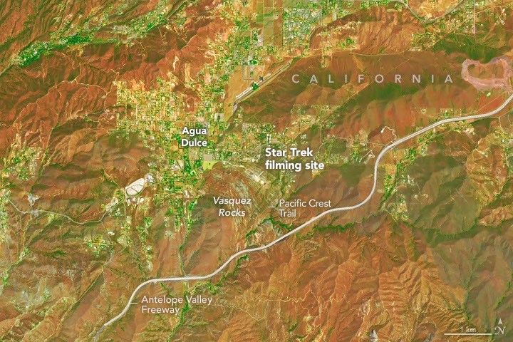
A zoomed-in view of the Vasquez Rocks part of the image highlights a sandy parking lot where Star Trek scenes were filmed, the Antelope Valley Freeway, and the nearby community of Agua Dulce.
Proximity to Los Angeles and the freeway is among the reasons the tilted strata at Vasquez Rocks have long been a popular filming location for television producers. This false-color image (bands 6-5-4) was captured by the OLI (Operational Land Imager) aboard Landsat 9 on July 28, 2026.
NASA Earth Observatory/Michala Garrison

The Vasquez Rocks didn’t start out pointing skyward. When they were forming 25 million years ago, sediment was spread across alluvial fans—cone-shaped deposits that develop as fast-moving streams empty onto relatively flat plains. The sediment likely hadn’t traveled far, much of it eroding from nearby uplands. Over time, the alluvial fan deposits were buried and cemented into thick layers of sandstone and conglomerate rock.

Over millions of years, the region was then reshaped by the interaction of tectonic plates just to the east. Two plates grind past each other along a boundary that includes the San Andreas Fault, a strike-slip fault where the North American plate moves southeast and the Pacific plate northwest, contributing to the powerful tectonic forces that ripple throughout the region.

Eventually this tectonic activity led to the uplift and deformation of the Soledad Basin, with sedimentary layers gradually tilting, folding, and rotating. Once they were exposed at the surface, millions more years of weathering and erosion sculpted the formations further, removing softer material and leaving the more resistant sandstone and conglomerate fins and ridges that wow visitors today.

The rock formations represent far-flung moons and planets in several other Star Trek episodes and Vulcan, Spock’s home planet, in two Star Trek movies. Other productions have highlighted the Vasquez Rocks as well. They make appearances in dozens of other television shows and movies, including the science fiction series Westworld, For All Mankind, and Battlestar Galactica.

NASA Earth Observatory images by Michala Garrison, using Landsat data from the U.S. Geological Survey. Story by Adam Voiland.

Downloads

In this false-color image, areas with more extensive vegetation on the Sierra Pelona retain more moisture than the hills surrounding Agua Dulce, making the Sierra Pelona appear dark green in comparison to the rusty brown coloration of the lower hills. Vasquez Rocks appears as a patch of curved gray stripes near the center of the image.

July 28, 2026: False color (bands 6-5-4)

JPEG (22.57 MB)

This natural-color image shows the same area, but there is less difference in colors between higher-elevation and lower-elevation vegetation. Most features in the image are shades of brown.

July 28, 2026: Natural color

JPEG (19.33 MB)

References & Resources

You may also be interested in:

Stay up-to-date with the latest content from NASA as we explore the universe and discover more about our home planet.

Digging Back in Time in the UAE

5 min read

Once below a shallow sea, Jabal al Fāyah now stands above the desert in the United Arab Emirates as a…

Article

What Lake Bonneville Left Behind

5 min read

The drying of the massive lake exposed playas that became the setting for feats of engineering and technological ingenuity, as…

Article

Pumice Rafts Encroach on Admiralty Islands

4 min read

Buoyant volcanic rock fragments from an underwater eruption drifted across the Bismarck Sea and choked island coasts.

Article

A Bright Spot at Mount Michael

7 September 2026 at 00:01
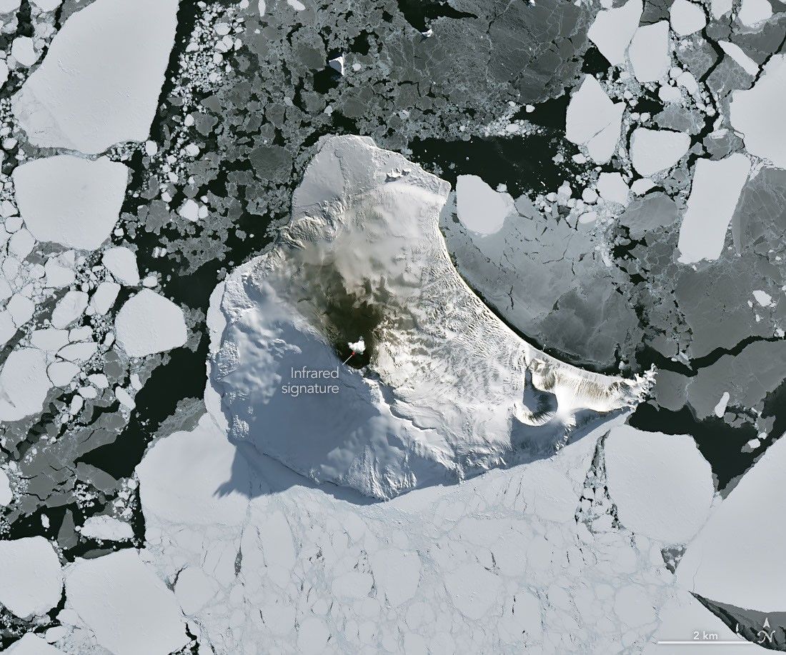
A small ice- and snow-covered island with an active volcanic crater at its center is surrounded by drifting pieces of sea ice. A thermal signal and small plume appear in the crater, and ash darkens the snow on the volcano’s northern slopes.
Mount Michael on Saunders Island, seen in this image acquired with the OLI (Operational Land Imager) on Landsat 8 on August 24, 2026, hosts a frequently active lava lake in its summit crater.
NASA Earth Observatory/Michala Garrison

Winter near the Antarctic Circle brings months of frozen darkness, when sea ice chokes ocean waters and many of its denizens hunker down to ride out the harsh conditions. But as winter began to release its icy grip, an uncommonly clear satellite image revealed that part of this remote realm was still very much awake, at least volcanically speaking.

Mount Michael, the stratovolcano at the center of Saunders Island, rises above the ice-filled South Atlantic Ocean in this image, acquired with the OLI (Operational Land Imager) on the NASA-USGS Landsat 8 satellite on August 24, 2026. The natural-color image is overlaid with an infrared signal (OLI bands 7-6-5), shown in red, revealing heat from the persistent lava lake in its summit crater. A puff of a volcanic plume hovering over the peak, along with darkened snow on its northern slopes, also suggests ongoing activity.

Saunders Island is one of the South Sandwich Islands, a string of small volcanic peaks about 350 kilometers (220 miles) long that formed from the South American plate subducting beneath the tiny South Sandwich plate. Regular eruptions, including at Mount Michael, have occurred on these islands in recent centuries.

Because of the volcanoes’ remoteness, scientists rely on satellite data to understand their activity. An analysis of thermal anomalies in Landsat, Sentinel, and ASTER (Advanced Spaceborne Thermal Emission and Reflection Radiometer) observations spanning 30 years led researchers to conclude that Mount Michael hosts a persistent lava lake in its summit crater. Only a handful of other volcanoes on Earth, including Kīlauea, Nyamulagira, and Erta Ale, are known to have similar, frequently active features.

Thermal observations from the MODIS (Moderate Resolution Imaging Spectroradiometer) and VIIRS (Visible Infrared Imaging Radiometer Suite) instruments have also enabled long-term monitoring of Mount Michael. Data provided through MIROVA, a near-real-time volcanic hot spot detection system, indicate that low-intensity activity has been ongoing at the volcano for the past several years. Other observations from NASA’s Aura satellite show that emissions of sulfur dioxide and other gases are common at Mount Michael.

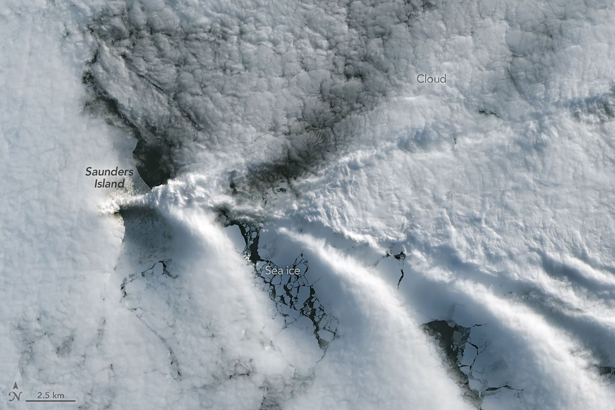
A series of V-shaped wave clouds appears over an ocean filled with pieces of sea ice.
Wave clouds form downwind of Saunders Island in this image acquired with the OLI (Operational Land Imager) on Landsat 9 on September 1, 2026.
NASA Earth Observatory/Michala Garrison

The cloud-free window over Mount Michael would close in short order. One week later, when Landsat 9 passed over the island, a more active atmosphere had returned. But the weather patterns interacted with the island to put on a spectacle of their own. The 843-meter-high (2,766-foot-high) peak jutting from the ocean disturbed passing winds to produce a series of wave clouds resembling the wake of a ship, a familiar phenomenon in this region. False-color imagery captured by NASA’s Aqua satellite indicates that a volcanic track caused by degassing sulfur dioxide was likely present as well.

NASA Earth Observatory images by Michala Garrison, using Landsat data from the U.S. Geological Survey. Story by Lindsey Doermann.

Downloads

A small ice- and snow-covered island with an active volcanic crater at its center is surrounded by drifting pieces of sea ice. A thermal signal and small plume appear in the crater, and ash darkens the snow on the volcano’s northern slopes.

August 24, 2026

JPEG (4.27 MB)

A series of V-shaped wave clouds appears over an ocean filled with pieces of sea ice.

September 1, 2026

JPEG (1.14 MB)

References & Resources

You may also be interested in:

Stay up-to-date with the latest content from NASA as we explore the universe and discover more about our home planet.

Ever Restless Mount Dukono Erupts

2 min read

The volcano on Indonesia’s Halmahera Island routinely ejects ash, volcanic gases, and volcanic bombs.

Article

A Sea of Spinning Clouds

3 min read

Icy, isolated Peter I Island stirred up a show in the atmosphere off the West Antarctic coast.

Article

America’s Emerald Isle

3 min read

Beaver Island is one in a string of verdant and scenic jewels in a northern Lake Michigan archipelago.

Article

Ice Island Survives Run-In With Joe Island

1 September 2026 at 00:00


AUGUST 24
AUGUST 23

A satellite view shows the iceberg after it pivoted out of the fjord into Nares Strait, wedged against a small, brown island.
NASA Earth Observatory / Lauren Dauphin

A satellite view shows a large tabular iceberg at the junction of its home fjord and Nares Strait.
NASA Earth Observatory / Lauren Dauphin

A satellite view shows the iceberg after it pivoted out of the fjord into Nares Strait, wedged against a small, brown island.
NASA Earth Observatory / Lauren Dauphin
A satellite view shows a large tabular iceberg at the junction of its home fjord and Nares Strait.
NASA Earth Observatory / Lauren Dauphin

AUGUST 24

AUGUST 23


An iceberg from Petermann Glacier encounters Joe Island in northwestern Greenland, visible in images captured by the OLI (Operational Land Imager) on Landsat 9 on August 23, 2026 (right), and August 24, 2026 (left). NASA Earth Observatory images by Lauren Dauphin.

Summer is prime iceberg season in Greenland’s glacier-fed fjords, and 2026 was no exception. Especially notable was the berg that broke from the Petermann Glacier along Greenland’s northwest coast in August. Roughly the size of St. Thomas in the U.S. Virgin Islands, it was the largest calving event by any Arctic glacier since 2020.

Iceberg calving is a routine part of an outlet glacier’s life cycle. Scientists watch the process closely, however, along with numerous other observations of the ice and its environment, for longer-term signs of instability. Petermann is one of Greenland’s largest marine-terminating glaciers and acts as a gatekeeper for ice flowing from the ice sheet into the ocean. Its future stability has implications for sea level rise.

The calving event of summer 2026 was spotted on August 4 by Adam Garbo, a doctoral student in glaciology at the University of Ottawa, in imagery from the European Space Agency’s Sentinel-1 mission. Garbo and an international team of colleagues have been using remote sensing to study and track the glacier’s ice tongue.

The team reported that the large tabular iceberg, or “ice island,” measured just over 76 square kilometers (29 square miles) at the time it calved—the largest to break from the glacier since the ice island of 2012 (130 square kilometers). The 2012 calving followed earlier major events in 2008 (31 square kilometers) and 2010 (just over 250 square kilometers).

The August 2026 event could have been even bigger. Garbo and colleagues had been expecting a major calving once one of the large rifts they were monitoring finally cut all the way across Petermann’s ice tongue. “What surprised us was that the calving instead followed a different fracture, producing a smaller ice island than we had originally anticipated,” Garbo said. As of late August, two large rifts remained and were expected to eventually produce new ice islands of roughly 94 square kilometers and 84 square kilometers, though the timing remained uncertain.

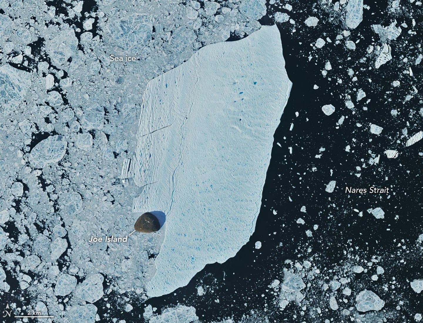
A detailed satellite view shows the iceberg wedged against the small, brown island, with sea ice packed densely to its left and more sparsely to its right.
August 24, 2026
NASA Earth Observatory/Lauren Dauphin

Glaciologist Mauri Pelto of Nichols College has also been tracking the iceberg, using images from NASA-USGS Landsat satellites, as it drifted down Petermann Fjord toward Nares Strait. In the week since it calved, the berg drifted an average of 3 kilometers per day. It continued toward the fjord’s junction with Nares Strait, where it rammed into a small rocky outcrop known as Joe Island (Joe Ø). The brief encounter is visible in images captured by the OLI (Operational Land Imager) on Landsat 9 on August 23 (top right) and August 24 (top left). A detailed view of the August 24 image is shown above.

Joe Island sits at the mouth of Petermann Fjord, making it one of the first obstacles a departing ice island meets. Collisions with it—like the one that split the 2010 ice island in two—often mark the start of a berg’s breakup. Petermann bergs tend to be thinner and more fragile than those calved by glaciers such as Greenland’s Jakobshavn and Helheim, and thinner still than Antarctica’s behemoths, Pelto noted.

“We were certainly watching closely as it interacted with Joe Island and were impressed that it survived the interaction without further fragmentation,” Garbo said.

The ice island was estimated to be less than 150 meters thick at the time of calving. Wind and surface currents have swept it out of the fjord, and satellite images show it pivoting away from Joe Island and continuing southwest through Nares Strait. As it drifts, it will fracture into smaller pieces as tides, winds, currents, and melting continue to weaken the ice.

Thicker bergs that calve from tidewater glaciers without floating ice-shelf extensions can drag and even become grounded on the seafloor within the fjord, while ice islands, like those from Petermann, might run aground later in their drift. Many ice islands have become “grounded” off the coasts of Coburg and Baffin islands.

Garbo and colleagues noted that ice islands and their fragments have been known to travel considerable distances, posing potential hazards to marine activities and infrastructure while also distributing freshwater through the ocean as they melt.

NASA Earth Observatory images by Lauren Dauphin, using Landsat data from the U.S. Geological Survey. Story by Kathryn Hansen.

Downloads

A satellite view shows a large tabular iceberg at the junction of its home fjord and Nares Strait.

August 23, 2026

JPEG (12.59 MB)

A satellite view shows the iceberg after it pivoted out of the fjord into Nares Strait, wedged against a small, brown island.

August 24, 2026

JPEG (10.23 MB)

References & Resources

You may also be interested in:

Stay up-to-date with the latest content from NASA as we explore the universe and discover more about our home planet.

Record-Setting Retreat of Hektoria Glacier

5 min read

Scientists relied on satellite data to understand how the Antarctic glacier lost so much ice so rapidly.

Article

Pasterze Hangs on as Austria’s Largest Glacier

4 min read

One narrowing icefall remains the linchpin for the Alpine glacier—and it may not be long for this world.

Article

An Uncommon Drifter in the Denmark Strait

4 min read

A large iceberg, observed in summer 2026, had drifted more than 1,000 kilometers south from the northeastern Greenland bay where…

Article

The Forested Floodplains of Congaree National Park

28 August 2026 at 00:01
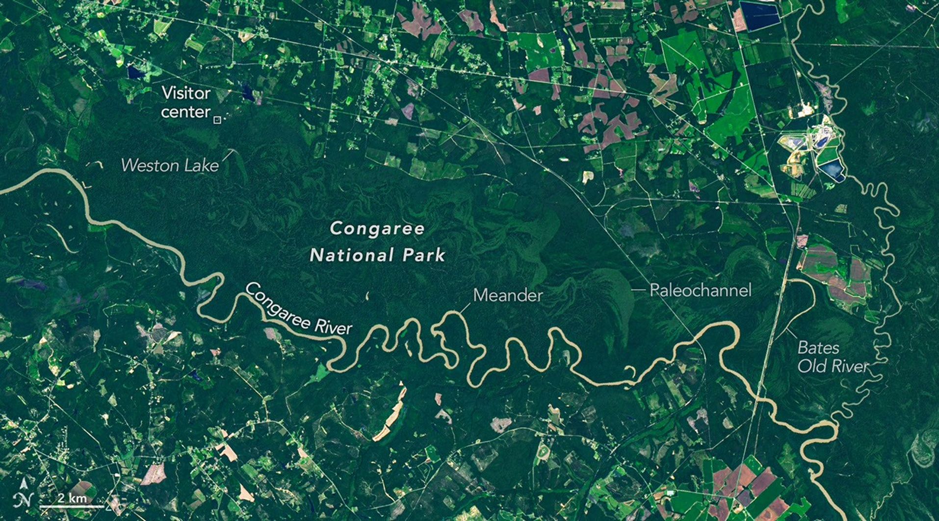
A brown, meandering river cuts through a band of dark green forest in Congaree National Park. Labels point out an oxbow lake and meander in the river. Former river channels called paleochannels appear lighter green than other forested areas.
The OLI on Landsat 9 captured this image of the Congaree River winding through floodplain forests in Congaree National Park on August 18, 2025.
NASA Earth Observatory/Michala Garrison

Among the 63 U.S. national parks, few are as defined by a single river’s floodplain as Congaree National Park in South Carolina. While the features are also prominent in other parks, a full 80 percent of Congaree National Park lies within the Congaree River floodplain.

It’s a place home to one of the largest intact tracts of old-growth bottomland hardwood forests in the United States. In this image captured by the OLI (Operational Land Imager) on Landsat 9, the river winds through the forested plain, along with curving bands of green that trace old channels, ridges, and swales left behind as the river gradually migrated across it. Slight differences in elevation in these paleochannels and other landforms affect how frequently they flood, producing distinct ecosystems that appear in contrasting shades of green.

The river flows through flat, soft terrain, which encourages the formation of bends and meanders. Water typically flows faster on the outside of bends, leading to more rapid erosion as the channel carves into the outer riverbank. It moves more slowly on the inside of bends, resulting in the deposition of sediment and the growth of sandy features called point bars. Over time, this process can cut off a bend from the main river channel, forming U-shaped oxbow lakes.

The National Park Service lists Weston Lake, 1.2 miles (1.9 kilometers) from the visitor center, as one of the park’s most permanent oxbow lakes, noting that it is relatively deep and lacks the shallow clay and silt layer found in most of the park’s other oxbow lakes, such as Devil’s Elbow. On the right side of the image is Bates Old River, a roughly 4-mile-long abandoned channel of the Congaree River and one of the longest oxbow lakes in South Carolina. Over time, abandoned channels and oxbow lakes can fill with sediment and become shallow wetlands. Some of these low-lying, water-filled features are known as sloughs, where flood-tolerant cypress-tupelo forests tend to grow.

While loggers targeted forests along the Congaree in the 1880s, challenges such as frequent flooding, interminably muddy roads, and mosquito-plagued conditions meant that most of the floodplain forests escaped the widespread logging that transformed other parts of the Southeast. By the 1950s, conservationists had begun to recognize how rare old-growth forests of this type had become in the region. Congress designated the area a national monument in 1976, and it became a national park in 2003.

As the river snakes its way through the park’s mostly flat terrain, it overflows its banks several times per year, usually in the winter and early spring but also in the summer and fall after hurricanes and major rainstorms. These floods distribute broad layers of nutrient-rich silt throughout the floodplain, nourishing the forests and contributing to the high concentration of unusually large trees in the park.

Over the decades, Congaree National Park has harbored a remarkable array of giant “champion” trees that have held national and state size records for their species. Though individual trees have gained and lost champion status as they have been damaged, have died, or been surpassed by newly measured trees elsewhere, Congaree trees such as the possumhaw (Ilex decidua), water hickory (Carya aquatica), loblolly pine (Pinus taeda), laurel oak (Quercus laurifolia), swamp tupelo (Nyssa biflora), and sweetgum (Liquidambar styraciflua) have held records at times.

During this National Park Week, celebrate by exploring Earth Observatory’s U.S. National Parks from Space collection. You can also check out the offerings of Earth to Sky, a collaborative program that connects NASA science with park service rangers across the nation.   

NASA Earth Observatory image by Michala Garrison, using Landsat data from the U.S. Geological Survey. Story by Adam Voiland.

Downloads

A brown, meandering river cuts through a band of dark green forest in Congaree National Park. Labels point out an oxbow lake and meander in the river. Former river channels called paleochannels appear lighter green than other forested areas.

August 18, 2025

JPEG (13.48 MB)

References & Resources

You may also be interested in:

Stay up-to-date with the latest content from NASA as we explore the universe and discover more about our home planet.

Minute Man National Historical Park

3 min read

Sites relevant to the start of the American Revolutionary War are interspersed throughout the modern-day Boston metropolitan region.

Article

Colonial National Historical Park

2 min read

The colonial communities of “America’s historic triangle” played defining roles in the road to American independence.

Article

Belts of Green in the Washington Suburbs

3 min read

Along the northeast side of the Capital Beltway in Maryland, green spaces weave through the developed landscape.

Article

A Changing World for Emperor Penguins

26 August 2026 at 00:01


1989
2025

In a satellite image captured in 1989, faint brown guano stains are visible on a background of white fast ice near a cluster of icebergs. The stains are near the edge of an ice shelf to the south.
NASA Earth Observatory/Michala Garrison

In a similar image captured in 2025, brown guano stains are still visible along the ice shelf, though the locations of icebergs.
NASA Earth Observatory/Michala Garrison

In a satellite image captured in 1989, faint brown guano stains are visible on a background of white fast ice near a cluster of icebergs. The stains are near the edge of an ice shelf to the south.
NASA Earth Observatory/Michala Garrison
In a similar image captured in 2025, brown guano stains are still visible along the ice shelf, though the locations of icebergs.
NASA Earth Observatory/Michala Garrison

1989

2025


Landsat has observed evidence of emperor penguins living on Smyley Island in Antarctica as early as 1989. The TM (Thematic Mapper) on Landsat 4 captured this false-color image (left) of guano stains on fast ice on December 24, 1989. The OLI (Operational Land Imager) on Landsat 8 captured a similar scene on December 10, 2025 (right). The images combine observations of infrared, red, and green light to make it easier to distinguish the guano stains. NASA Earth Observatory images by Michala Garrison.

With their charming waddles, heat-conserving huddles, and tuxedo-like plumage, emperor penguins are among the world’s most recognizable animals. Recent satellite surveys estimate that hundreds of thousands of the flightless birds live in 66 colonies spread around Antarctica’s inaccessible, frozen coastlines. But those numbers could fall in the coming decades because emperor penguins rely on landfast (or fast) ice—a type of sea ice attached to the shoreline—to breed, raise chicks, and molt.

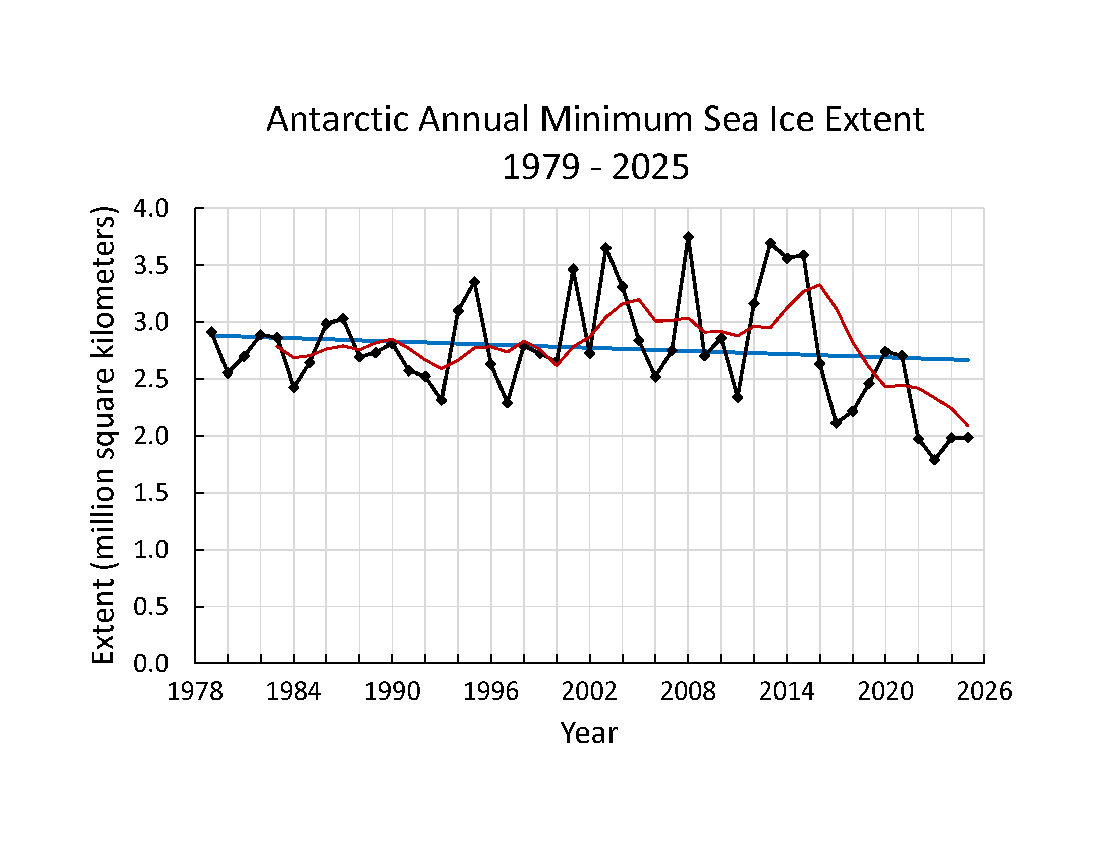
While Antarctic sea ice remained relatively stable between the late 1970s and 2015, it has been declining since 2016, and climate projections suggest that trend will continue. How landfast ice is faring remains poorly understood and is an active area of study. However, one study suggests that it has declined in West Antarctica and the Weddell Sea in recent decades even as it has trended upward in the Bellingshausen Sea and East Antarctica.  

Meanwhile, some models project that emperor penguins could disappear by 2100 due to their habitats becoming inhospitable. The U.S. Fish & Wildlife Service listed emperor penguins as threatened in 2022, and the International Union for Conservation of Nature classified them as endangered in 2026.

After Antarctic sea ice cover hit a record low in 2022, British Antarctic Survey researchers reported “catastrophic” breeding failures among Bellingshausen Sea colonies. However, new research, based on decades of observations from NASA-USGS Landsat satellites, offers some hope, underscoring that many colonies have persisted for decades and that emperor penguins may be more flexible about where they breed than previously thought.

Except for a few well-studied colonies, scientists have known little about how long many emperor penguin colonies have existed, how their populations have changed, or how they have responded to past disruptions in landfast sea ice.

Three adult penguins with black-and-white plumage are surrounded by several younger penguins with fuzzy gray plumage.
Adult and juvenile emperor penguins congregate on sea ice in Antarctica.
Michael Van Woert, NOAA NESDIS, ORA

“There’s little baseline information for what’s ‘normal’ for most of these colonies,” said Michelle LaRue, a wildlife ecologist at the University of Canterbury. That’s made projecting future population levels a challenge.

Two new studies published in 2026 used decades of Landsat observations to start filling gaps in understanding. Landsat cannot resolve individual penguins, but researchers identify colonies from the guano stains that accumulate where thousands of birds congregate on the ice.

Using this technique, researchers at the University of Freiburg found that 18 colonies predate their initial identification by an average of 17 years. Because Landsat has imaged Antarctica continuously since the early 1980s, it provides one of the few systematic long-term records of remote penguin colonies.

Among the oldest colonies studied was the roughly 6,000-bird Smyley Island colony in the Bellingshausen Sea, which dates to at least 1989, two decades earlier than previously known. Other colonies that predated their earliest known presence by 20 or more years included those at Barrier Bay, Brownson, Luitpold Coast, Ragnhild, Smith, and Verdi Inlet.

Scientists have watched the Smyley Island colony closely in recent years because it is among the colonies that may have suffered a total breeding failure in 2022. Satellite images captured that year show the colony splitting up, with some penguins moving onto a large iceberg grounded near the coast.

Despite persistently low sea-ice conditions since then, the colony has continued to appear in satellite imagery, generally establishing itself near icebergs along the edge of the ice shelf. The image above on the right shows the colony in December 2025, the most recent month Landsat has observed the colony.

“We’re seeing a degree of resilience in the Smyley Island colony,” LaRue said. “They seem to be doing okay now, and we will continue to monitor them to learn more about their behaviors.” The colony’s persistence underscores that one bad breeding year—even a total failure—doesn’t mean the end of a colony. Blizzards and predators can lead to bad years with very low chick survival rates as well, she added. “It’s when we start to see frequent breeding failures year after year that the birds won’t be able to keep up, and it starts to be a problem for a colony.”

An image (left) shows a long trail of guano extending from rift ice northward to a larger guano stain on a nearby ice shelf in 2018. In 2023, brown guano stains are visible on fast ice much closer to open water, while there is no sign of the penguin colony on the ice shelf (right).
Landsat 8 captured an image of the SANAE colony with a guano trail leading from rift ice to the ice shelf on January 23, 2018 (left). On January 4, 2023, the birds had returned to their original fast ice area (right). The images combine observations of infrared, red, and green light to make it easier to distinguish the guano stains.
NASA Earth Observatory/Michala Garrison

A second study, led by Grant Macdonald, a remote sensing scientist at Durham University, found further evidence of behavioral flexibility. Macdonald and colleagues analyzed nearly 40 years of observations from Landsat, the ASTER (Advanced Spaceborne Thermal Emission and Reflection Radiometer) on NASA’s Terra satellite, and other sources for three colonies disrupted by iceberg calving or early sea ice breakup. They found that penguins of the Mertz and SANAE colonies responded by temporarily shifting to nearby icebergs, embayments, or ice shelves before returning to their former breeding sites.

Landsat first imaged the SANAE colony in 1984 on fast ice in a sheltered bay in the Queen Maud Land region in East Antarctica. After a major calving event in 2011 exposed the fast ice to more punishing winds, the colony relocated to rift ice in an embayment 11 kilometers (7 miles) to the south. The move proved temporary. Part of the group moved to another nearby site, and part of it returned to the original breeding location in 2016.

Yet in the 2016–2017 breeding season, the returnees did something unexpected. Despite the presence of stable fast ice, they trekked onto the ice shelf and huddled and bred there. In the Landsat image above, a winding guano-stained trail traces the penguins’ route onto the ice shelf. By 2022, after roughly a decade of wandering and splitting between sites, the entire colony had returned to its original breeding ground on the fast ice, where it has bred each year since.

At the third colony the researchers studied, the Astrid colony on the Vigridisen Ice Shelf, the birds kept returning to their original breeding location even after a major calving event in 2006. That’s likely because some fast ice remained and nearby icebergs provided some shelter. The guano stains indicate that the colony did, however, sometimes spend time on a nearby ice shelf toward the end of the breeding season both before and after the calving event.

Indeed, moving and sometimes breeding on alternative surfaces such as ice shelves, icebergs, or rift ice may be “more common and feasible than previously thought,” Macdonald said, perhaps because some sites offer better shelter from wind. This willingness to move may represent a “useful adaptation” as ocean temperatures warm and sea ice declines, he added, though he cautioned that behavioral flexibility alone won’t necessarily offset the long-term effects of continued sea-ice loss.

“We have so much more to learn about emperor penguins,” added LaRue. “These colonies are so remote and difficult to access that satellites—especially government satellites with easily accessible data—are going to be absolutely invaluable to understanding what the future will bring for them.”

NASA Earth Observatory images by Michala Garrison, using Landsat data from the U.S. Geological Survey. Photo by Michael Van Woert (NOAA NESDIS, ORA). Story by Adam Voiland.

Downloads

In a satellite image captured in 1989, faint brown guano stains are visible on a background of white fast ice near a cluster of icebergs. The stains are near the edge of an ice shelf to the south.

December 24, 1989

JPEG (5.26 MB)

In a similar image captured in 2025, brown guano stains are still visible along the ice shelf, though the locations of icebergs.

December 10, 2025

JPEG (2.67 MB)

An image (left) shows a long trail of guano extending from rift ice northward to a larger guano stain on a nearby ice shelf in 2018. In 2023, brown guano stains are visible on fast ice much closer to open water, while there is no sign of the penguin colony on the ice shelf (right).

January 23, 2018

JPEG (4.15 MB)

An image (left) shows a long trail of guano extending from rift ice northward to a larger guano stain on a nearby ice shelf in 2018. In 2023, brown guano stains are visible on fast ice much closer to open water, while there is no sign of the penguin colony on the ice shelf (right).

January 4, 2023

JPEG (6.85 MB)

References & Resources

You may also be interested in:

Stay up-to-date with the latest content from NASA as we explore the universe and discover more about our home planet.

Pink Penguin Guano Provides Diet Clues

3 min read

The color of Adélie penguin droppings reveals what the birds are eating, offering scientists a way to track how sea…

Article

Record-Setting Retreat of Hektoria Glacier

5 min read

Scientists relied on satellite data to understand how the Antarctic glacier lost so much ice so rapidly.

Article

An Uncommon Drifter in the Denmark Strait

4 min read

A large iceberg, observed in summer 2026, had drifted more than 1,000 kilometers south from the northeastern Greenland bay where…

Article

An Uncommon Drifter in the Denmark Strait

20 August 2026 at 00:00
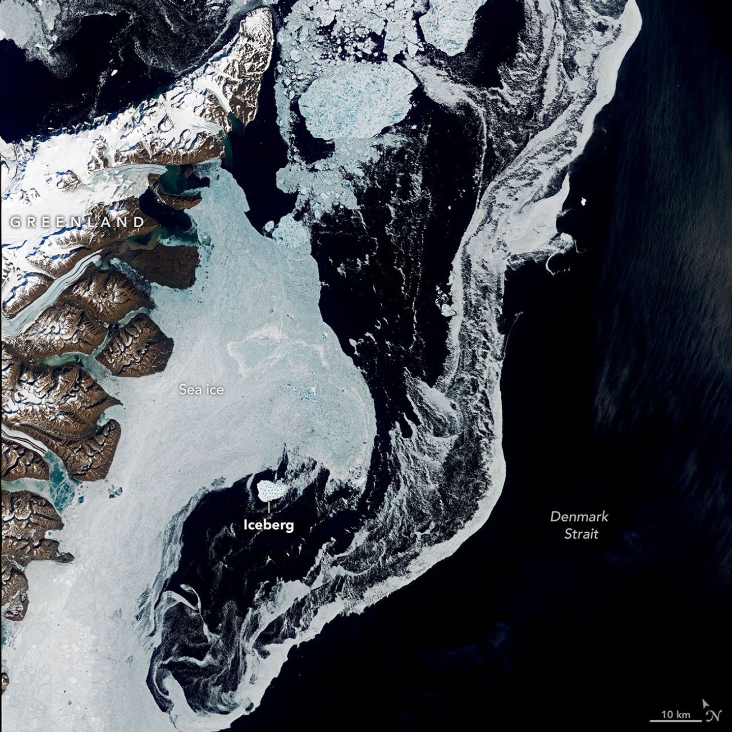
A satellite image shows the dark blue waters of the Denmark Strait with swirling sea ice to the right of eastern Greenland. A bright white iceberg sits amid the sea ice in the middle-left of the scene.
An iceberg drifts through the Denmark Strait in this image acquired on June 12, 2026, by the OLI (Operational Land Imager) on Landsat 9.
NASA Earth Observatory/Lauren Dauphin

Greenland’s jagged coastline is lined with fjords, many of them cradling marine-terminating glaciers that routinely calve icebergs into the water. It’s common to see these bergs, small and large, drifting in the island’s fjords each summer once the sea ice breaks up. In summer 2026, one exceptionally large berg turned up in the Denmark Strait—more than a thousand kilometers south of where it apparently originated. 

These images, captured by the OLI (Operational Land Imager) on Landsat 9, show the iceberg on June 12 as it drifted in the strait between Greenland and Iceland. It was just south of Kangikajiip Appalia, a cape on Greenland’s east coast visible in the scene’s upper left, amid a mixture of sea ice and berg fragments known as “mélange.”

Alexis Denton, oceanographer and chief scientist with the International Ice Patrol, noted that several clues indicate it is an iceberg rather than thick, multi-year sea ice: its proximity to shore, its whiter color, and larger size compared to the surrounding sea ice. Measuring roughly 17 square kilometers (7 square miles) on June 12, the iceberg was about five times the area of New York City’s Central Park. That’s modest compared to the behemoth bergs that calve from Antarctic glaciers and ice shelves but large by Greenland standards.

Keld Quistgaard, a senior ice advisor with the Danish Meteorological Institute’s Greenland Ice Service, noted that it originated in Jøkelbugten—a bay in northeastern Greenland. The berg’s precise origin within that bay, however, remains something of a mystery. It’s possible that the berg broke off from Zachariæ Isstrøm or its adjacent remnant ice shelf. The ice shelf, which together with Zachariæ Isstrøm once filled the bay, was abandoned after the glacier rapidly retreated in the early 2000s.

Tracing its path back through satellite imagery is challenging. Through spring, the bay and surrounding coastal areas are choked with sea ice and berg fragments, making individual bergs hard to distinguish, especially if covered in bright snow. In late May, for instance, the berg was surrounded by numerous look-alikes. Only later in the season, as it drifted farther south and the ice around it thinned out, did it become distinct enough to easily spot.

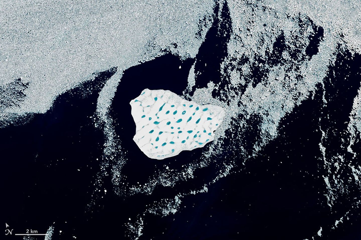
A detailed view shows the iceberg's bright white surface pocked with light blue meltwater ponds. Broken pieces of sea ice float around the iceberg in otherwise dark blue ocean water.
The iceberg’s bright white surface is pocked with light blue meltwater ponds in this detailed view of the image, acquired on June 12, 2026, by the OLI (Operational Land Imager) on Landsat 9.
NASA Earth Observatory/Lauren Dauphin

Its size and striking network of blue meltwater ponds offer some clues to its origin, according to Christopher Shuman, a retired University of Maryland glaciologist. Shuman thinks the berg broke from the remnant ice shelf rather than the glacier itself. Bergs calved from Zachariæ Isstrøm tend to be smaller, he said. Also, the berg’s surface—pocked with meltwater ponds, “like Swiss cheese”—closely resembles the remnant shelf ice. Past satellite images show pieces of that shelf ice drifting south and getting trapped among islands bordering the bay, where winds and tides have jostled them for years.

As of mid-August, the berg was about 1,500 kilometers (900 miles) from the bay, drifting south on the Greenland Coastal Current into the North Atlantic. Quistgaard expected the iceberg to gradually disintegrate throughout the month. Recent satellite imagery suggested it was doing just that.

Breaking up in the Denmark Strait means that remnants of the berg are unlikely to drift into busier shipping lanes that go past the southern tip of Greenland. “Its journey is a reminder of the dynamic Earth,” Shuman said, “as well as the seasonal variability of the ice in this part of the North Atlantic.”

NASA Earth Observatory images by Lauren Dauphin, using Landsat data from the U.S. Geological Survey. Story by Kathryn Hansen.

Downloads

A satellite image shows the dark blue waters of the Denmark Strait with swirling sea ice to the right of eastern Greenland. A bright white iceberg sits amid the sea ice in the middle-left of the scene.

June 12, 2026

JPEG (16.74 MB)

References & Resources

You may also be interested in:

Stay up-to-date with the latest content from NASA as we explore the universe and discover more about our home planet.

Record-Setting Retreat of Hektoria Glacier
5 min read

Scientists relied on satellite data to understand how the Antarctic glacier lost so much ice so rapidly.

Article
A Bare Summer for Barnes Ice Cap
4 min read

The expanse of glacial ice on Canada’s Baffin Island lost its snow cover quickly and early in summer 2026, revealing…

Article
Pink Penguin Guano Provides Diet Clues
3 min read

The color of Adélie penguin droppings reveals what the birds are eating, offering scientists a way to track how sea…

Article

Stops Along the Path of Totality

12 August 2026 at 00:01
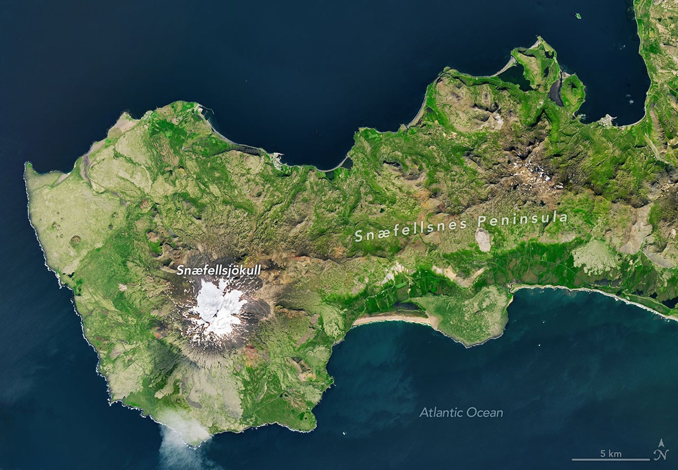
A peninsula in Iceland stretches across the image to the left. A prominent glacier-capped volcano sits near its western end.
The glacier-capped Snæfellsjökull volcano is the defining feature of Iceland’s Snæfellsnes peninsula, shown in this image acquired with the OLI (Operational Land Imager) on Landsat 9 on July 25, 2026.
NASA Earth Observatory/Michala Garrison

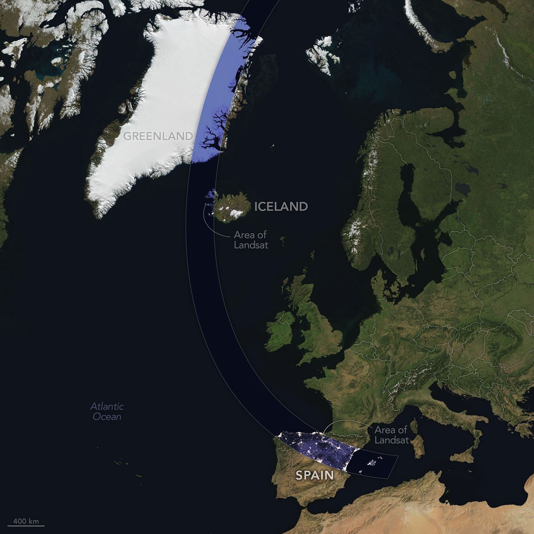
The Sun, Moon, and Earth align on August 12, 2026, to produce a total solar eclipse. When this celestial event last occurred, on April 8, 2024, the path of totality stretched across North America, giving millions the chance to glimpse the Sun’s corona. In 2026, the viewing locales are more limited; only a handful of land areas in the Northern Hemisphere, including parts of Iceland and Spain, fall within the path of totality.

On August 12, the Moon’s shadow will first cross over the Arctic Circle from northern Russia and then track along the eastern side of Greenland. At about 5:45 p.m. local time in Iceland (17:45 Universal Time), the country’s western fringes—including the Snæfellsnes peninsula, shown in the Landsat image above—will begin to experience totality. The greatest eclipse will occur near this sparsely populated peninsula when the Moon appears the largest and covers more of the Sun.

A map shows the path of totality of the solar eclipse on August 12, 2026, arcing across Greenland, Iceland, the North Atlantic, and Spain.
The path of totality of the solar eclipse on August 12, 2026, spans Greenland, Iceland, and Spain. The base imagery for the map comes from Blue Marble: Next Generation, with data from Black Marble shown in the path of totality. Blue Marble is built from scenes captured by MODIS (Moderate Resolution Imaging Spectroradiometer), while Black Marble is based on observations by the VIIRS (Visible Infrared Imaging Radiometer Suite) day-night band.
NASA Earth Observatory/Michala Garrison

The Snæfellsjökull volcano on the western end of the peninsula is covered in ice and last erupted about 1,800 years ago. It is the highlight of a national park of the same name, where people are expected to visit to view the eclipse. The stratovolcano even has a literary claim to fame: in Jules Verne’s A Journey to the Center of the Earth, characters venture underground through its crater, later emerging in an eruption of Stromboli, in Italy. In 2025, a broader area of the peninsula was designated a UNESCO biosphere reserve, containing over 70 percent of Iceland’s flora and an agglomeration of volcanic landscapes, wetlands, and grasslands.

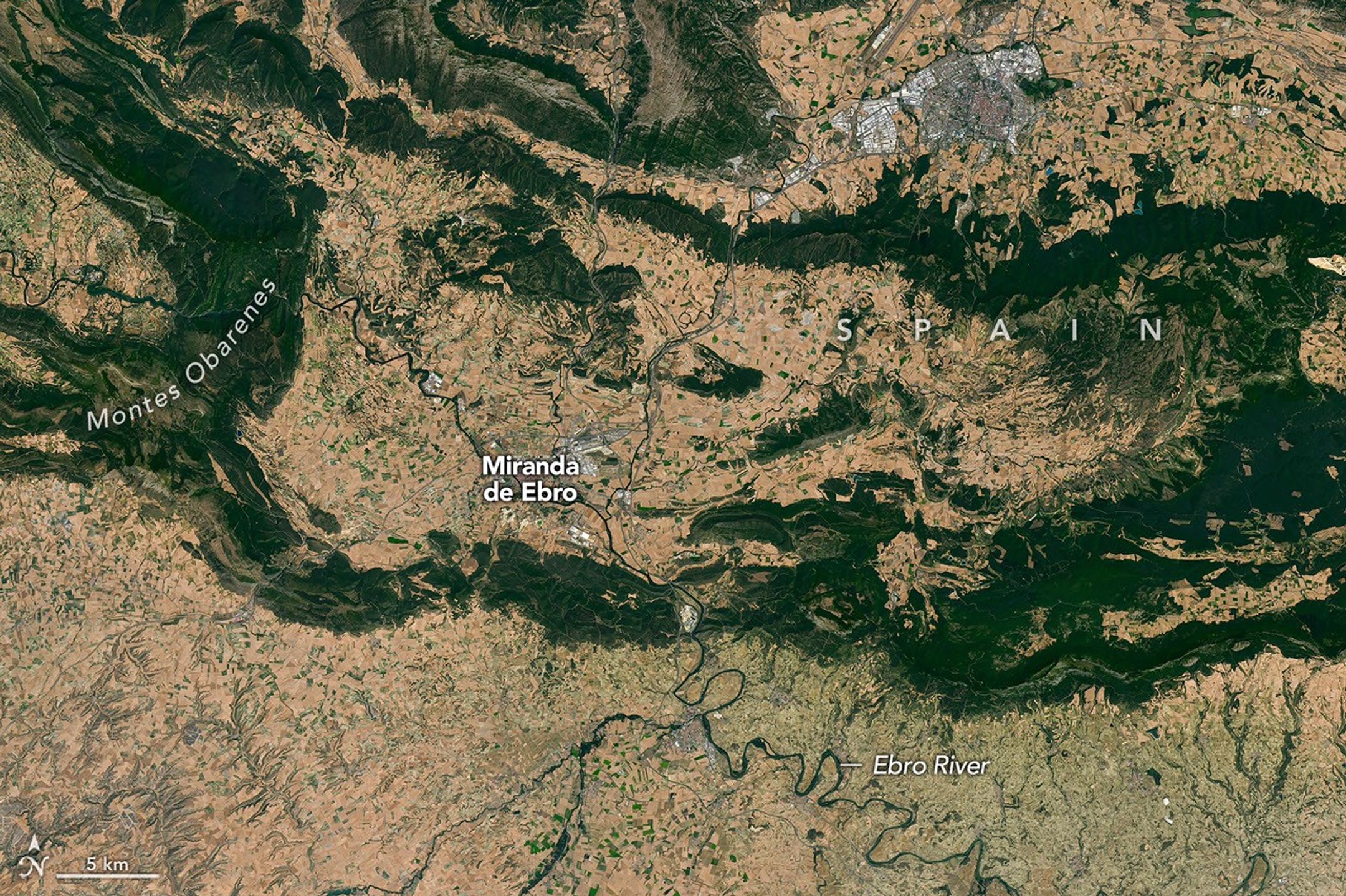
From Iceland, the eclipse shadow, or umbra, progresses across the North Atlantic and reaches northern Spain shortly before sunset. It runs east-southeast across the country, much like the Ebro River (Río Ebro), seen in the Landsat image below.

Meandering rivers cut through dark green mountain ridges, across agricultural land, and near several developed areas in northern Spain.

The Ebro River, meandering across northern Spain in this image acquired with the OLI (Operational Land Imager) on Landsat 8 on July 21, 2026, is in the path of totality of the August 2026 solar eclipse.
NASA Earth Observatory/Michala Garrison

The upper Ebro emerges from rugged terrain in Parque Natural de Montes Obarenes-San Zadornil, where it carves canyons and gorges through the eastern foothills of the Cantabrian Mountains. It then meanders through La Rioja, a region known for its vineyards. About 400 kilometers (250 miles) away, the river reaches a delta on the Mediterranean coast between Barcelona and Valencia.

Based on satellite measurements of cloud cover in August over several decades, viewers in Spain have a higher likelihood than those in Iceland of getting a clear look at the eclipse. And despite limited viewing opportunities in the path of totality, the rest of Europe, parts of Africa, Canada, and the northern and northeastern U.S. will experience a partial eclipse.

NASA Earth Observatory images and map by Michala Garrison, using Landsat data from the U.S. Geological Survey, base imagery from Blue Marble: Next Generation and Black Marble, and eclipse path data from Xavier Jubier. Story by Lindsey Doermann.

Downloads

A peninsula in Iceland stretches across the image to the left. A prominent glacier-capped volcano sits near its western end.

July 25, 2026

JPEG (14.69 MB)

A map shows the path of totality of the solar eclipse on August 12, 2026, arcing across Greenland, Iceland, the North Atlantic, and Spain.

August 12, 2026

JPEG (1.92 MB)

Meandering rivers cut through dark green mountain ridges, across agricultural land, and near several developed areas in northern Spain.


July 21, 2026

JPEG (34.46 MB)

References & Resources

You may also be interested in:

Stay up-to-date with the latest content from NASA as we explore the universe and discover more about our home planet.

Colonial National Historical Park

2 min read

The colonial communities of “America’s historic triangle” played defining roles in the road to American independence.

Article

Minute Man National Historical Park

3 min read

Sites relevant to the start of the American Revolutionary War are interspersed throughout the modern-day Boston metropolitan region.

Article

Earthset From the Lunar Far Side

2 min read

The crew of NASA’s Artemis II mission captured extraordinary images of our home planet during their journey around the far…

Article

How the Tide Turns at the Mouth of the Elbe

6 August 2026 at 00:01


August 15, 2025
May 11, 2025

The Elbe river in Germany into the North Sea on the left side of the image. Low tide exposes wide, light-colored tidal flats interrupted by branching channels of dark water.
The ocean’s ebbs and flows reveal dynamic tidal flats and a well-traveled shipping route along the German coast.
NASA Earth Observatory/Lauren Dauphin

The Elbe river in Germany into the North Sea on the left side of the image. At high tide, a handful of small islands and crescent-shaped sandbars remain exposed above the water level near shore. Ships are visible as small, bright specks on the water.
The ocean’s ebbs and flows reveal dynamic tidal flats and a well-traveled shipping route along the German coast.
NASA Earth Observatory/Lauren Dauphin

The Elbe river in Germany into the North Sea on the left side of the image. Low tide exposes wide, light-colored tidal flats interrupted by branching channels of dark water.
The ocean’s ebbs and flows reveal dynamic tidal flats and a well-traveled shipping route along the German coast.
NASA Earth Observatory/Lauren Dauphin
The Elbe river in Germany into the North Sea on the left side of the image. At high tide, a handful of small islands and crescent-shaped sandbars remain exposed above the water level near shore. Ships are visible as small, bright specks on the water.
The ocean’s ebbs and flows reveal dynamic tidal flats and a well-traveled shipping route along the German coast.
NASA Earth Observatory/Lauren Dauphin

August 15, 2025

May 11, 2025


One of the major rivers of Europe, the Elbe flows more than 1,000 kilometers (600 miles) across the continent before reaching the North Sea. At its mouth, the low-lying landscape is continually reshaped by the rise and fall of the tides. These dynamic tidal flats are a boon to biodiversity while sometimes posing challenges for those navigating its waters and for communities living along its shores.

The images above illustrate how the area changes with the tides. They were acquired on August 15, 2025, at low tide (left) and on May 11, 2025, at high tide (right) with the OLI (Operational Land Imager) on Landsat 9. The mean tidal range at Cuxhaven is 2.9 meters (9.5 feet), which is considered intermediate, or mesotidal. The tides are also asymmetrical, meaning the flood period is shorter than the ebb. This causes the incoming current to run faster and typically carry more sediment up the 140-kilometer-long (87-mile-long) estuary than it does out.

The low tide exposes complex channels, sandbars, and mudflats around the river mouth. This wide zone of coastal wetlands is part of the Wadden Sea, which stretches from the Netherlands to southern Denmark and represents the largest continuous system of intertidal sand and mud flats in the world. Its habitats serve as important staging, molting, and wintering grounds for migratory birds, with more than 10 million passing through every year.

A channel cuts through these natural features near the river’s mouth, allowing ships to reach Cuxhaven and Hamburg—the third-largest container port in the European Union—farther upriver. Dredging is required to remove accumulated sediment in the channel, and some ships can only pass through when the tide is high enough. The Elbe’s mouth also provides access to the Kiel Canal, which connects the North Sea and Baltic Sea and is the world’s busiest human-made waterway navigable by seagoing ships. 

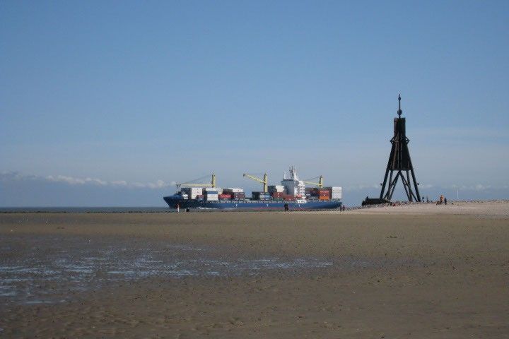
A broad tidal mudflat fills the foreground of this photo.  A sliver of deeper water is visible on the horizon, where a cargo ship loaded with shipping containers and cranes appears to be traveling to the left.
A cargo ship passes by mudflats at the mouth of the Elbe.
Thomas Gölles, April 5, 2009.

At high tide (right), only a handful of small islands and sandbars remain above the waves. One of these islands, Neuwerk, is a tranquil tourist destination that is home to a few dozen inhabitants and the oldest building on the German coast. A brick tower, completed in 1310 and later converted to a lighthouse, was built to protect shipping on the Elbe from pirates and wreckers.

These images show normal tidal variation in the area, but storms can push water levels much higher than a typical high tide. The highest water level measured at Cuxhaven—5.1 meters (16.7 feet) above Europe’s official sea level reference—occurred on January 3, 1976, when a fast-moving storm swept across the North Sea and slammed the coast with high winds. Researchers who reconstructed historical storms noted that the storm surge was worsened by its timing relative to the tide. The strongest winds arrived around low tide, preventing water that had propagated upstream at high tide from flowing back out to sea and causing further inundation inland.

Scientists study past extreme events like this to better understand how future storms might affect low-lying coastal areas and how flood protection could be improved. Flooding risks can be exacerbated by rising sea levels, which at Cuxhaven have trended upward by 2.12 millimeters per year, or 0.70 feet per century.

Two new Earth-observing satellites are making it possible to measure water levels in coastal areas in greater detail. The dual-band radar on the NISAR (NASA-ISRO Synthetic Aperture Radar) satellite is expected to track long-term phenomena such as sea level changes, as well as to map flood inundation and other ephemeral events. In addition, early data from NASA’s SWOT (Surface Water and Ocean Topography) satellite has demonstrated the potential to accurately measure water levels around complex coastlines and to improve tidal models.

NASA Earth Observatory images by Lauren Dauphin, using Landsat data from the U.S. Geological SurveyPhoto by Thomas Gölles. Story by Lindsey Doermann. 

Downloads

The Elbe river in Germany into the North Sea on the left side of the image. Low tide exposes wide, light-colored tidal flats interrupted by branching channels of dark water.

August 15, 2025

JPEG (6.33 MB)

The Elbe river in Germany into the North Sea on the left side of the image. At high tide, a handful of small islands and crescent-shaped sandbars remain exposed above the water level near shore. Ships are visible as small, bright specks on the water.

May 11, 2025

JPEG (6.02 MB)

References & Resources 

You may also be interested in:

Stay up-to-date with the latest content from NASA as we explore the universe and discover more about our home planet.

A Tide-Fueled Trove of Biodiversity in Guinea-Bissau

3 min read

The expansive mudflats, sandy beaches, and mangrove forests of the Bijagós archipelago support an array of migratory shorebirds and large…

Article

Signs of Thaw in the Bering Sea

3 min read

Drifting sea ice fragments near Alaska’s Saint Lawrence and Nunivak islands and colorful water around the Yukon Delta heralded the…

Article

Barents Sea Tied to Low Arctic Sea Ice

4 min read

Patches of open water in the region contributed to low sea ice extent across the Arctic in March 2026, which…

Article
❌
❌