 Login
LoginGPOD on the Road: Piet Oudolf’s Sculpture Garden at Singer Laren
11 September 2026 at 03:00
At Singer Laren, Piet Oudolf’s layered plantings create a living backdrop for contemporary sculpture


Usually in Tech In Plain Sight, we talk about technology you probably see every day, even if you don’t notice it. But we hope you don’t get to see one of the latest crop of medical robots, such as the LUCAS chest compression system. If you watch the popular TV series “The Pitt”, though, you may have caught a glimpse of one of these medical marvels. They aren’t fiction. They are very real devices.
Calling them robots might be stretching the definition a little. They don’t roam the halls looking for patients. But once attached to someone in cardiac arrest, they can take over one of the most important — and physically demanding — parts of CPR: chest compressions.
When someone’s heart stops pumping blood, time is critical. CPR doesn’t normally restart the heart on its own. Instead, chest compressions produce enough blood flow to keep oxygen reaching the brain and heart while rescuers work on the underlying problem and, when appropriate, use a defibrillator.
Doing that well is harder than it looks on television. Current American Heart Association guidelines call for adult chest compressions 100 to 120 times per minute, at least 5 cm deep but generally no deeper than 6 cm, while allowing the chest to recoil fully between compressions. Interruptions should be kept to a minimum.
That’s hard physical work. In fact, studies show compression depth begins to fall after only about 90 to 120 seconds, which is one reason CPR teams normally swap compressors every two minutes. But a robot doesn’t get tired.
LUCAS stands for Lund University Cardiopulmonary Assist System, reflecting the device’s origins in Lund, Sweden. Early versions entered clinical use around 2002-2003 and were pneumatically powered. Later versions replaced the compressed-gas system with an electric motor and battery.
The current LUCAS 3 looks something like a small drill press straddling the patient as you can see in the video below. A backplate goes beneath the torso, and a frame locks onto it. An electrically driven piston presses a suction-cup-like pad against the sternum. Internally, the motor drives a belt and ball screw that moves the piston up and down.
Factory settings are around 102 compressions per minute and roughly 53 mm compression depth for a typical adult, although parameters can be configured.
Beyond tirelessness, another obvious advantage is that LUCAS doesn’t need hands. Medics can deal with ventilation, drugs, defibrillation, IV access, and the dozens of other things occurring during a cardiac arrest. More importantly, the device can keep compressing while a patient is being carried, wheeled through corridors, or transported in an ambulance — situations where doing good manual CPR is awkward and sometimes dangerous to the practitioner.
You might reasonably expect perfectly regular machine CPR to beat a tired human. Large randomized trials haven’t demonstrated that, however. The 4,471-patient PARAMEDIC trial found 30-day survival of 6.3% with LUCAS versus 6.8% with manual CPR, not a statistically significant difference. The 2,589-patient LINC trial similarly found essentially identical four-hour survival — 23.6% versus 23.7% — and no significant improvement in longer-term neurological outcomes.
That doesn’t make the machines useless. It says something slightly different: high-quality mechanical CPR hasn’t proven superior to high-quality manual CPR as a routine replacement. The International Liaison Committee on Resuscitation currently recommends against routine mechanical CPR, while specifically noting that it can be a reasonable alternative when sustained manual compressions are impractical or would endanger the practitioner.
One issue is setup. Installing the machine adds a time penalty: compressions must stop briefly while the backplate and mechanism are positioned. Good training is essential to keep that interruption short. Another problem is that some studies show potential links to higher rates of internal chest injuries, such as bleeding around the lungs. There have also been rare device malfunctions or power failures that can compromise care.
LUCAS isn’t alone. ZOLL’s AutoPulse takes a very different mechanical approach. Instead of a piston pushing on one spot, a motor tightens a broad load-distributing band around the patient’s chest.
There’s also the German corpuls cpr, which returns to the piston idea but uses a cantilevered single-arm mechanism. That leaves much of the chest unobstructed and makes the system useful during procedures such as cardiac catheterization.
So perhaps these aren’t quite the autonomous robot doctors science fiction promised us. But when your heart has stopped, and a machine is tirelessly pumping your chest a hundred times a minute while the medical team works around it, you probably won’t complain. We hope you don’t have to find out.
We’ve seen DIY devices, though certifying medical devices for actual use isn’t for the faint of heart. Robots can also help train humans to do better CPR.
Featured image is a still from the instructional video “Physio-Control LUCAS 3 Chest Compression System – Hospital Use” by MFI Medical.
A few weeks ago, my wife was out walking the dog, and she sent me four or five photos of small orange boxes planted all around our neighborhood. (OK, I’ll bite!) They had little cards on them explaining that they were geophones, and a QR code on them that lead to a website with all the details. Munich was getting a large-scale seismic survey to map out our underground water, with the aim of using it for geothermal heat and power in the near future.
How do you map up to five kilometers under the earth? You pound the ground, sending shockwaves downward, and then listen for their reflections. At the boundaries between different layers, the change in the speed of sound in the different media cause reflections. Calculating the time it took for a given reflection to reach you lets you figure out how deep the layer boundary is.
The seismic survey procedure goes like this: geophones are set out at roughly 20 m intervals in lines spaced around 300 m apart that run roughly north-south, while “vibrotrucks” drive a roughly east-west course, creating mini-earthquakes every 20 meters along the way. Covering a surface of 1,000 km^2 with over 120,000 sample locations and exciting them 86,000 times is going to take a while. Lucky for me, they started in my part of town.

Because the earth is essentially a ball of hot molten metal with a thin and crispy outer crust, and because there is radioactive decay going on even within the crusty bit, temperatures rise as you dig down: roughly 30 °C per kilometer. And Munich has this fantastic source of water that’s folded under the earth in a layer that dates back to the Jurassic, which makes it both low in dissolved minerals and sitting just around 3 km down: at 100 °C. This turns out to be the sweet spot in terms of difficulty of drilling and heat gained from doing so.
Blessed with hot water underground, the question is how to best use it. The plan at the moment is to situate a number of geothermal plants around the city, drill relatively large bore holes at each site that reach down 1 km to 2 km, and then drill diagonally down after that to spider out into a larger source of water. This “extended reach drilling” pulls from a larger heat source, prevents cool spots, and has only recently become technologically feasible.
Which brings us to the GIGA-M study. A 3D map of the underground will help plan out where to put the geothermal plants, in which directions the runners will need to be drilled, and generally how to best coordinate the resource. There were a number of individual smaller surveys done over the last 20 years, and Munich and the surroundings already have a number of geothermal plants, but this survey aims to fill in all of the gaps.
It was a Thursday morning when my wife thought she heard some pounding and humming outside. She was wrong, but it got us to look at the online map, and while they weren’t in our neighborhood just yet, they were probably within easy driving distance. I threw my camera and tripod in the car and headed out.

Out in the country, just outside of Grossdingharting (you can’t make these names up!) I spotted a plume of dust rising up from a field. Was it just a farmer tilling? Or was it a vibrotruck? I drove through the woods on a logging road, and when I came out, I was nearly face-to-face with the beasts.
They were loud, and I felt the rumble when I stepped out of the car, so I ran up and asked if I could film it. They said “sure”, and I set up the tripod. The first video I shot, apparently I hadn’t screwed the camera down hard enough in the tripod, and it vibrated loose. So I ran another 20 m further and tightened everything down.
I’m not going to lie: it was exceedingly loud and very exciting. I drove back home and couldn’t wait to review the footage.
The next morning, I heard the same sound outside my own house. They were driving vibrotrucks around in the field about a block up the street. I grabbed the camera and ran out barefoot to get footage. And then Saturday morning, while cooking blueberry pancakes for the family, they drove up my street. Am I stalking the vibrotrucks, or are they stalking me?
An engineer asked if they could stand in our front yard, so I took my chance to bombard him with questions. He seemed stoked to talk about it.
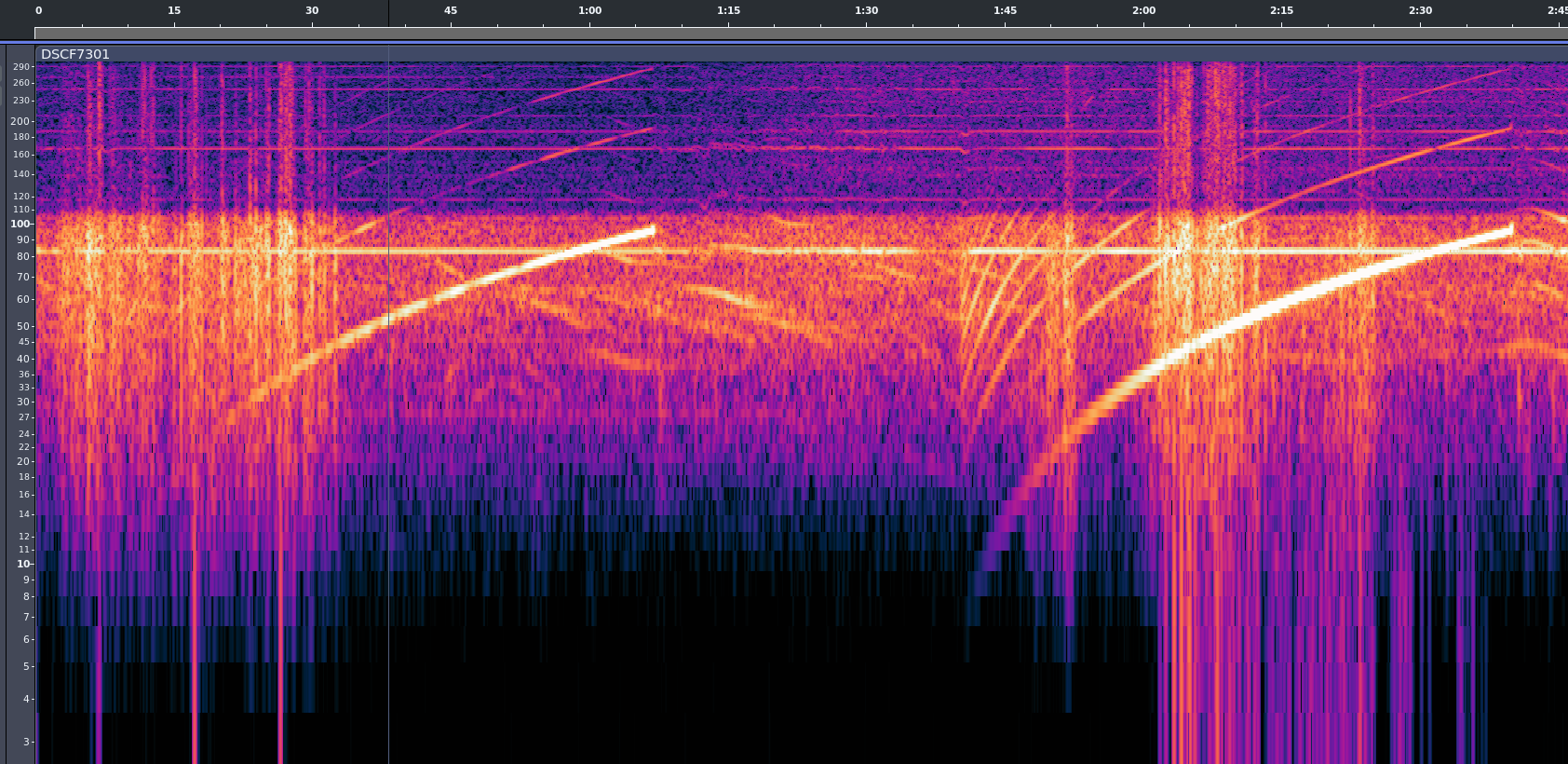 When you stand next to one of these things, first it shakes, and then you can hear a bassy tone, and then it rises and stops. They’re obviously doing a frequency sweep, much like you would use a sonar chirp to help disentangle the multiple reflections from one another.
The sweep means that even if they receive two reflections at once, they will hear two different pitches because one signal traveled further than the other, and comes from the earlier, lower-pitch part of the impulse. It also makes for a very easy to find signature. Correlating these times of flight across the entire array of geophones gives a 3D map of the underground layer discontinuities.
You can see from a cleaned up version of the audio that they’re sweeping from something like 6 Hz up to maybe 96 Hz. The lower end sounds like distinct hammering, and the top end a humming. Here is another video, with filtered audio. Because you feel the vibrations through your feet and in your chest, the live experience is a little bit like this with more noise. Play on good headphones or with a subwoofer for maximum effect.
Of course, the time of flight matters. I asked if each geohpone had a GPS timebase, and the friendly engineer told me that they individual geophones don’t – too expensive – but that when they install one, they connect it to a laptop with GPS that records the location and sets the geophone’s clock. When they harvest them, they record the location again, dump the time to verify that the clocks haven’t drifted too much, and then pull down all of the recorded timestamped data.
Why do they drive around in pairs? It’s simply because they make twice the vibration. The two trucks are actually synced together in phase, so they emit as one. The trucks have a GPS-disciplined clock inside, so they know exactly when they start each cycle and can derive the time-of-flight to all of the receiving geophones. The rest is math.
He also mentioned that it was too bad that I only got to experience the smaller “urban” vibrotrucks like the one outside my house. I kept my mouth shut – nobody needs to know that I’m a vibrotruck stalker.
If you used a scientific calculator in the 1970s or 1980s, there was a fair chance that it worked differently from almost every calculator you see today. Instead of typing:
2 + 3 =
you entered:
2 ENTER 3 +
There wasn’t even an equals key. Hewlett-Packard made this system — Reverse Polish Notation, or RPN — practically synonymous with serious scientific calculators until other players like TI and Casio got serious. Once you got used to it, ordinary algebraic calculators could feel annoyingly clumsy.
Today, RPN calculators look like a nearly extinct species. HP left the calculator market, licensing the HP calculator line to Moravia Consulting. Old HP-15Cs, 16Cs, 32Ss, 42Ss, and 48s have become collectibles. But RPN isn’t dead. You can still buy new hardware, build your own, or turn almost any computer or phone into a very capable RPN machine. There are reasons some of us still want to.
The name goes back to Polish logician [Jan Łukasiewicz], who devised a notation in which operators precede their operands. Instead of writing:
A + B
you can write:
+ A B
The big advantage is that parentheses aren’t required. The structure of the expression tells you exactly what operates on what. Reverse Polish notation simply puts the operator at the other end:
A B +
[Łukasiewicz] wasn’t designing calculators, of course, but the same idea turned out to be extremely convenient for computers and calculators. Your software doesn’t have to remember what operation is in progress. Each operator is ready to go and can simply work on the operands that you’ve already read.
RPN isn’t exactly the way people calculate with pencil and paper, and it certainly wasn’t derived from the slide rule, but there is a similarity in the way you work. With a slide rule, you generally establish some value, operate on it, and continue from the result. When doing a long-hand calculation, you often calculate a subexpression, write down the answer, and use that answer in the next step. You will probably start with the inner parenthesis and work outward, just like someone with an RPN calculator does. RPN formalizes that process with a stack.
Suppose you want:
(3 + 4) × (5 + 6)
On a conventional calculator, you either need parentheses, or you have to calculate one result and remember it. On an RPN calculator:
3 ENTER

4 +

5 ENTER

6 +

×
The first + leaves 7 on the stack. The second leaves 11 above it. The multiply consumes both and leaves 77.
Notice what’s missing: parentheses, an equals key, and any need to tell the calculator about precedence. This isn’t much of a win for a five-key calculation. It becomes more apparent with something like computing the value of a bunch of parallel resistors:
R=1/(1/R1+1/R2+1/R3…)
An RPN user can calculate each reciprocal, add it to the running result on the stack, and finally take the reciprocal. Intermediate answers stay in the calculator naturally instead of being stuffed into memory registers or enclosed in increasingly impressive collections of parentheses.
Is RPN better? Calculator users have been arguing about that for half a century. But once RPN gets wired into your fingers, it can be surprisingly hard to give up.
Although RPN and HP are nearly inseparable in popular memory, HP didn’t invent the RPN calculator. That distinction generally goes to the Friden EC-130, introduced in 1964. It was a 44-pound transistorized desktop calculator costing $2,150, and its CRT actually displayed all four levels of its RPN stack at once. More than 18,000 were eventually made. You can even simulate it in Verilog, if you like.
HP entered the business in 1968 with the HP 9100A, a programmable desktop scientific calculator. It weighed about 40 pounds and sold for $4,900, but it provided logarithms, trigonometry, hyperbolic functions, coordinate conversion, programming, and RPN operation. HP famously called it a calculator rather than a computer partly because customers could often buy calculators without getting corporate computer departments involved.
Then came the machine that changed everything: 1972’s HP-35, the first HP pocket scientific calculator. From there, RPN became a defining characteristic of HP calculators for decades.
There were financial calculators, programmer’s calculators, scientific calculators, graphing calculators, and eventually the RPL machines such as the HP-28 and HP-48, which generalized the stack idea into an entire programming environment.
Eventually, though, algebraic entry won the mass market. Even HP began producing machines with algebraic modes, and some later calculators let you choose either system.
So did RPN die out? Are there any RPN machines left in 2026? Quite a few, as it turns out. The real question is do you want a calculator that pretends, in some way, to be your favorite old-fashioned RPN calculator, or do you want a more modern device that happens to use (or, at least, is able to use) RPN?
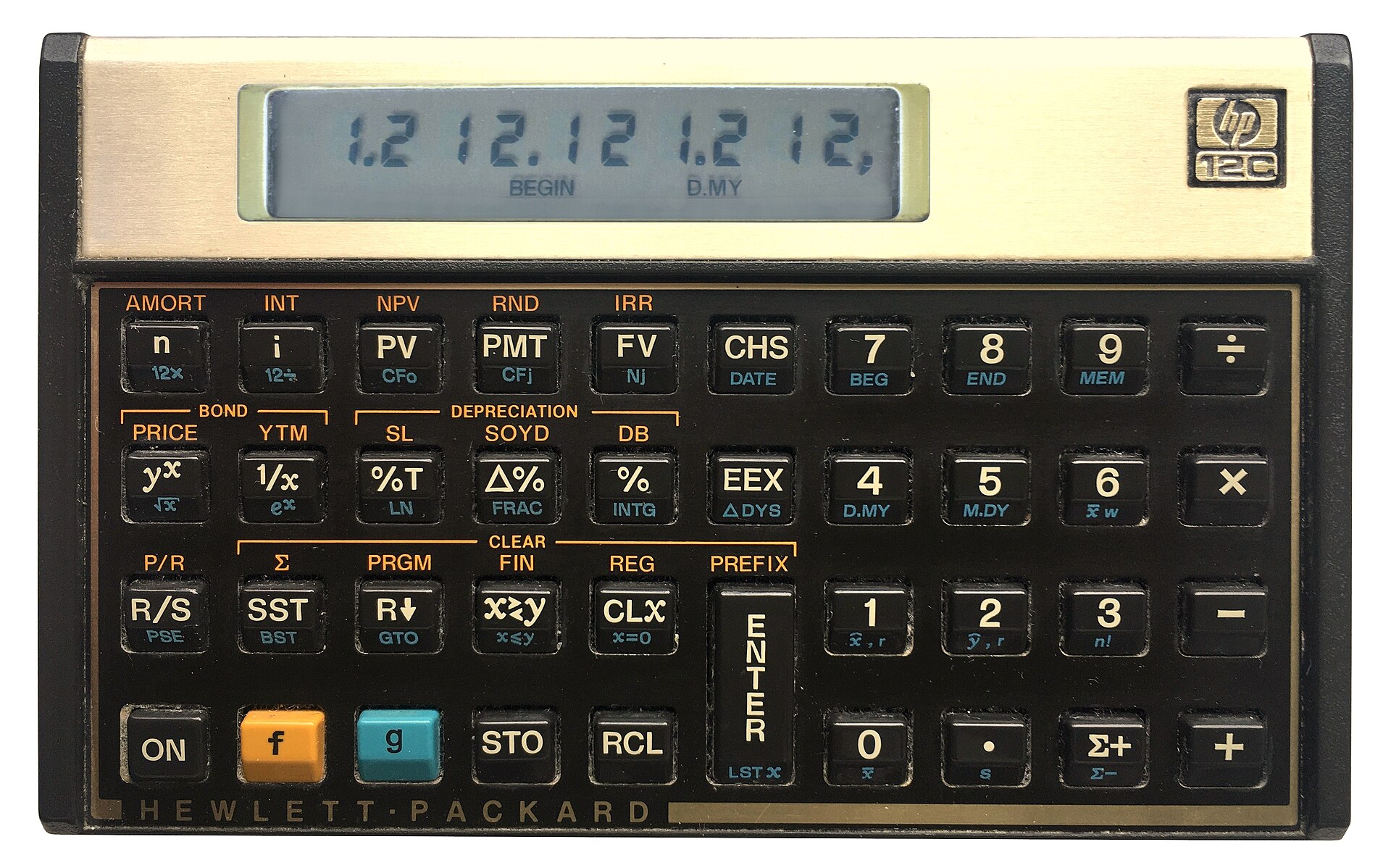
The strange survivor is the HP-12C. Introduced in 1981 as a financial calculator, it remains available new more than four decades later. Depending on the retailer, expect something around $50 to $70. The 12C Platinum, which can operate in either RPN or algebraic mode, is also still available for roughly $80 to $110.
Then there is the HP Prime G2, generally around $150 to $170. The Prime is a graphing calculator with CAS, programming, symbolic mathematics, touch screen, and textbook-style input — but buried among all of that is an RPN entry mode. It isn’t an old-fashioned HP RPN calculator, but it certainly qualifies.
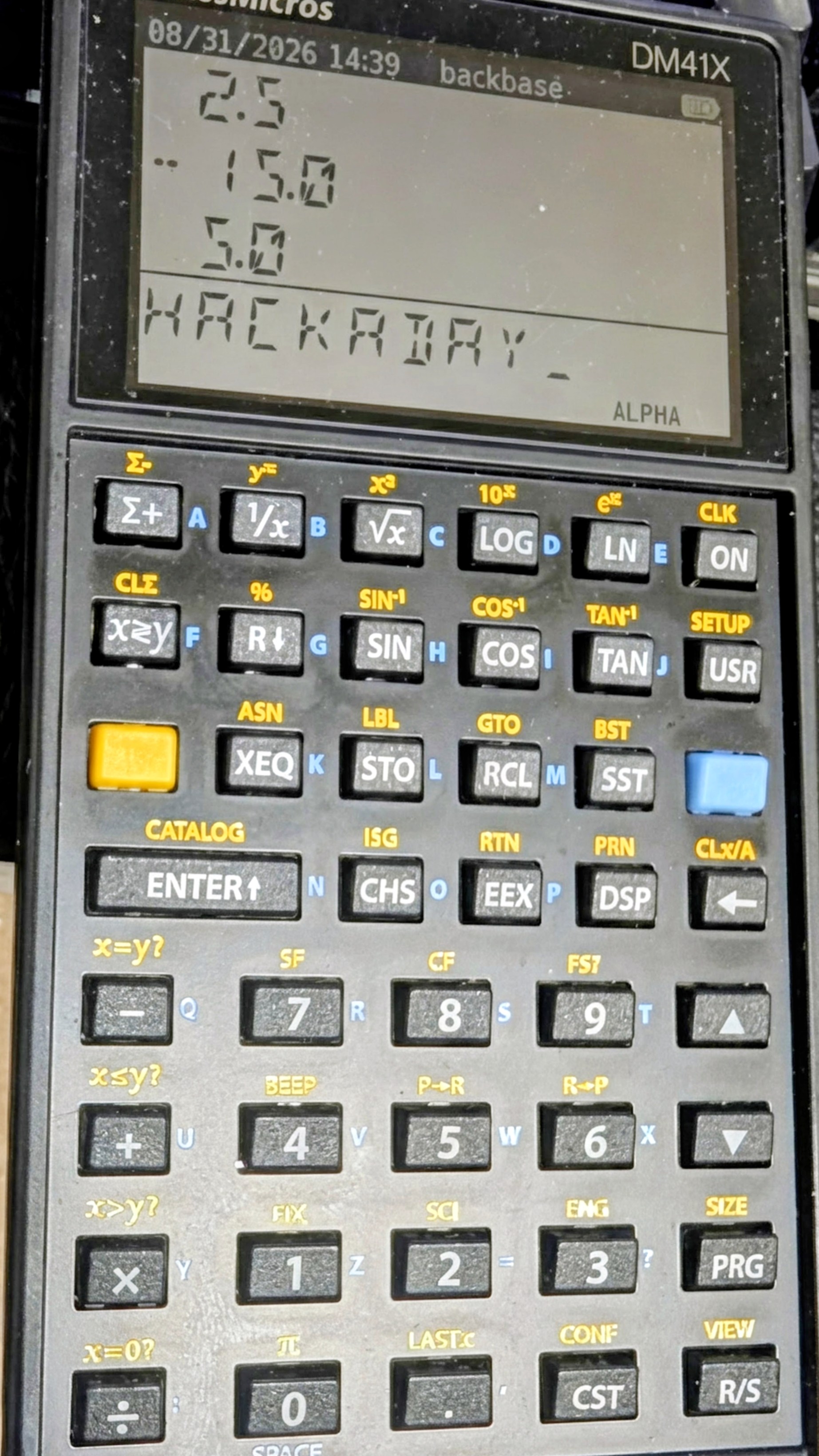
The real center of new RPN hardware today, however, is SwissMicros. SwissMicros started by producing modern implementations of classic HP designs and has since moved well beyond simple reproduction. Its current machines include the DM15L, modeled after the HP-15C; the DM16L programmer’s calculator; DM41L, DM41C, and DM41X machines inspired by the HP-41 family; and the DM32, which occupies roughly the territory once covered by the HP-32SII.
Perhaps more interesting is the R47, at about the same price. Instead of recreating a particular HP calculator, it grew out of the WP34S/WP43 community projects and attempts to be a modern enthusiast’s RPN calculator. It has an eight-level stack, matrices and vectors, complex arithmetic, base-N and bit operations, statistics, units, financial calculations, equation solving, integration, programming, and even built-in electrical engineering functions. Its firmware is still officially considered beta. This is probably the closest thing today to somebody asking, “What calculator would an obsessive HP engineer build if we started over?”
SwissMicros calculators aren’t cheap. Depending on the model, you’re generally looking at roughly $180 to more than $300 after currency conversion. But they are real, currently manufactured calculators rather than 40-year-old collectibles.
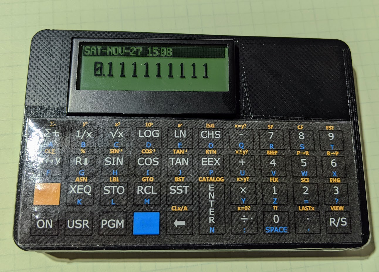
The ATmega scans the keyboard, drives the display, and emulates the original machine. The design adds such modern amenities as continuous memory, an LCD backlight, real-time clock, and considerably higher execution speed than the originals. Kits and assembled versions are typically under $100.
There is also the 10LC (and related models), which approaches the problem from the other direction: take inexpensive ESP32-based M5Stack Cardputer hardware, add calculator firmware and key labels, and turn the whole thing into a pocket RPN calculator. Figure roughly $50-$60.
It isn’t going to make a calculator collector forget an HP-42S keyboard, but it does show how little hardware is actually required to build an extraordinarily capable calculator today.
CalcTastic is a modern RPN phone app.If physical keys aren’t mandatory, RPN is actually thriving. You can get a host of RPN calculators on your Android or iPhone. There are many options for desktop computers, too. You can generally find these on your platform’s program repositories.
One of the best places to start is Free42, [Thomas Okken’s] free, clean-room implementation of the HP-42S. It runs on Android, iOS, Windows, macOS, and Linux. Plus42, from the same author, takes that foundation and expands it with equations, units, directories, plotting, financial functions, and other capabilities that the original HP-42S never had.
Android users also have CalcTastic, which can switch between algebraic and RPN modes and provides scientific calculation, complex numbers, fractions, statistics, conversions, and — in the paid version — programmer functions. The basic version is free, and the Plus version is only a few dollars.
For the HP-48 crowd, there is Droid48 on Android and several HP-48 implementations on iOS. If your idea of a calculator includes directories, symbolic objects, programs, lists, and an RPL command line, the phone in your pocket can impersonate a 48 far faster than the original hardware ever could. If you prefer the HP41C, go41C is the one I like.
Apple users have an especially large selection. i41CX recreates and extends the HP-41 environment. PCalc isn’t primarily an RPN calculator, but has long offered a very good RPN mode. There are also modern RPN calculators including MathU, RPN Calc, RPN Calculator 48, and a growing number of simulations of individual classic HP machines.
Even HP’s current flagship environment is available in software. HP Prime Pro runs on Android and iOS and supports optional RPN input.
Desktop users aren’t left out either. HP provides a free HP Prime Virtual Calculator for Windows, and there has also been a macOS version. Most unusually, HP once produced an actual native Linux version. The Linux release was packaged as an AppImage and survives as a 2019 technical preview — build 2.1.14288 in the copy sitting on my Linux machine. It isn’t the Windows version hidden inside Wine; it’s a native HP build, and it still works remarkably well. Unfortunately, it predates one particularly interesting addition to the Prime: Python programming.
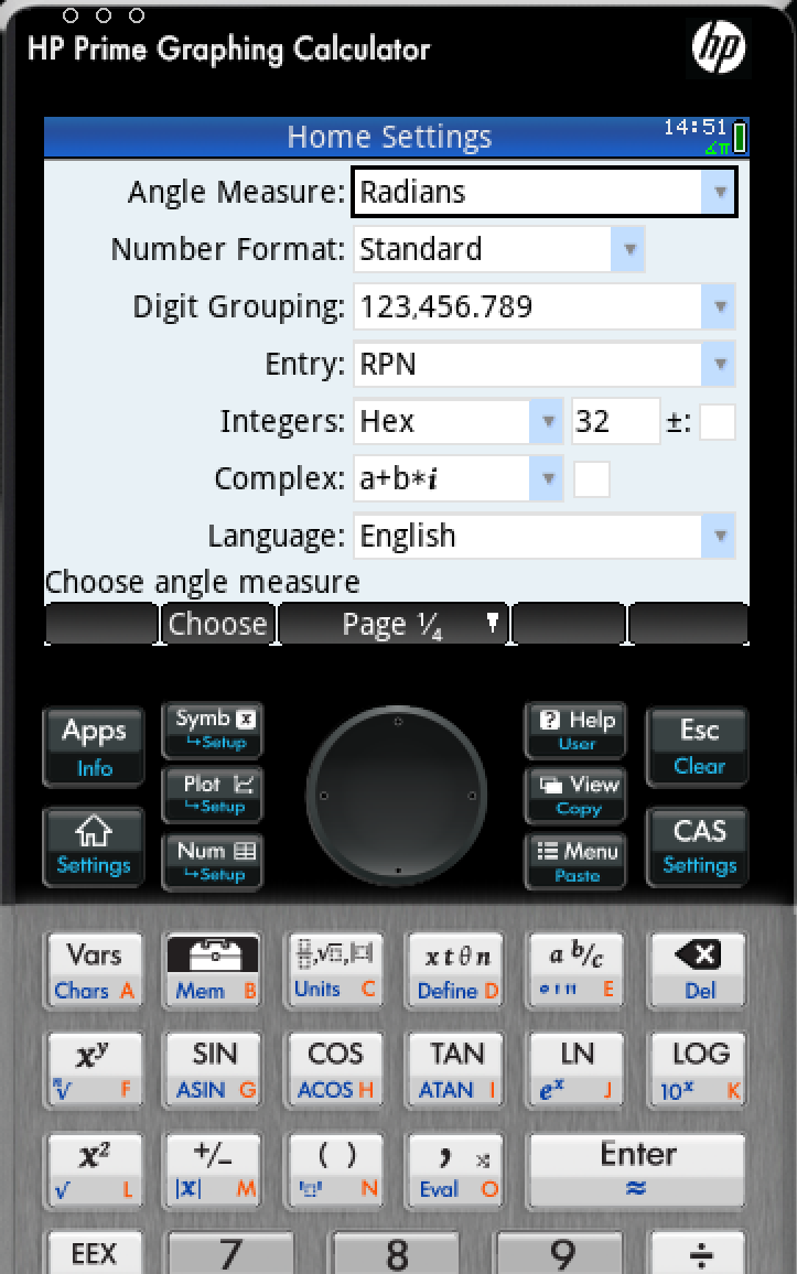
There is a way to get that on Linux, although HP doesn’t make it easy. I found that the December 2024 Windows release of the Virtual Calculator, version 2.2.15212, runs under Wine using the Soda 9 runner in Bottles. That version includes the Prime’s Python app and reports MicroPython 1.9.4. The catch is that you don’t want to accept its offer to upgrade. Updating to the current Windows version causes the simulator to stop working under the same setup, and Soda 11 doesn’t appear to fare any better. So there is a slightly absurd sweet spot where an older Windows Prime under an older Wine runner provides a more up-to-date Prime on Linux than HP’s own native Linux build.
Between Free42, Plus42, Prime, HP-48 emulators and innumerable smaller projects, software may actually be the easiest way to use RPN today.
Of course, another source is available: millions of old calculators are already out there. If you’ve always wanted an HP-11C, 15C, 16C, 28S, 32SII, 41CX, 42S, or 48GX, auction sites and used-equipment dealers will happily provide one. Sometimes you can still find a bargain, especially if you’re willing to buy a cosmetically ugly machine or something outside the most desirable models. The problem is that the best old calculators aren’t merely used calculators anymore. They’re collectibles.
A calculator that originally lived in an engineer’s shirt pocket may now be a pristine example with its case, manuals, and box — and priced accordingly. Even fairly ordinary examples of desirable models can sell for enough money that carrying one around every day starts to feel irresponsible. My treasured HP41C, for example, works fine, but is already scuffed up enough that I rarely risk using it at my desk these days.
That creates a slightly absurd situation. A perfectly functional 35- or 40-year-old calculator may cost considerably more than an astonishingly capable modern computer because one is being priced as a collectible and the other as a tool.
On the other hand, battered calculators exist. If you don’t care about scratches, engraved names, missing battery doors, or someone’s old asset-control sticker, those are often exactly the machines to buy. You’re going to use it, after all.
RPN plainly lost the calculator wars. Walk into an office supply store, and almost every calculator on the shelf expects conventional algebraic input. But it didn’t disappear.
You can still buy an HP-12C. You can buy sophisticated new RPN machines from SwissMicros. You can solder together your own HP-inspired calculator around an 8-bit AVR. You can turn an ESP32 gadget into one. Or you can install an app and have an HP-42S, HP-48, or modern RPN calculator in your pocket for anywhere from nothing to a few dollars.
That’s a surprising amount of life for an input system the mainstream calculator industry decided we didn’t want decades ago. Then again, people who like RPN tend to really like RPN.
If 2 ENTER 3 + looks more natural to you than 2 + 3 =, apparently somebody is still willing to sell you a calculator. If you want to see how easy it can be to parse RPN in a program, we’ve done that.
If you tear into old TVs or recording equipment, you may see shields made from some exotic-looking metal. Old timers will tell you it’s called mu metal, and its purpose is to — sort of — shield things from magnetic fields. The qualification is important. Unlike a conductive RF shield, mu metal doesn’t really stop a magnetic field. Instead, it gives magnetic flux an easier path to follow around whatever you’re trying to protect.
Mu metal belongs to a family of soft magnetic nickel-iron alloys. A typical modern formulation is about 80% nickel and 15% iron, with molybdenum and a few other elements making up most of the remainder. What makes it useful is its extremely high magnetic permeability. Commercial material can have relative permeability around 100,000 or more, and some specialty alloys can reach even higher.
You can think about reluctance as the magnetic equivalent of resistance. Put a high-permeability shell around something sensitive, and magnetic flux would much rather travel through the shell than through the space inside it, just like current tends to take the path of least resistance.
This works particularly well for DC and low-frequency fields, exactly where your usual copper or aluminum EMI shield isn’t much help.
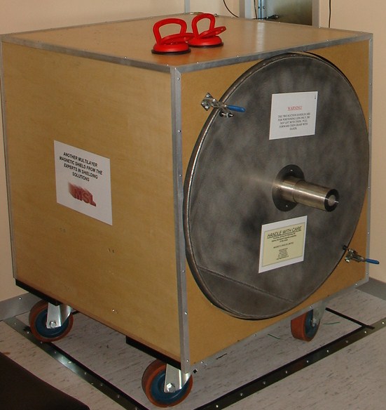
However, mu metal is still around. Modern applications include magnetometers, precision current sensors, electron microscopes, scientific instruments, and experiments that require extremely low magnetic fields. Commercial multi-layer mu-metal chambers are still sold for creating near-zero-field environments; with suitable construction and degaussing, some claim attenuation of static and low-frequency fields by factors approaching a million.
Quantum and cryogenic instrumentation have also created some 21st-century magnetic shielding problems. Ordinary mu metal loses performance at very low temperatures, so related nickel-iron alloys are made specifically for operation at liquid-nitrogen and liquid-helium temperatures.
There are a couple of catches. First, mu metal gets much of its impressive permeability from its metallurgical structure. Machining, stamping, welding, or even bending it can introduce stresses and seriously degrade its magnetic properties. High-performance shields are therefore commonly formed first and then hydrogen annealed to restore their permeability.
So buying a sheet of wonderfully permeable material and folding it into a box isn’t necessarily the recipe for a wonderfully permeable box.
The second surprise is saturation. Mu metal is superb with weak fields but isn’t necessarily what you want closest to a powerful magnet. Its saturation induction is only around 0.75 tesla. In strong fields, manufacturers recommend combining it with a lower-permeability material having higher saturation capability, letting that outer layer tame the field before the mu metal handles what’s left.
British scientists Willoughby S. Smith and Henry J. Garnett patented mu metal in 1923 for inductive loading of submarine telegraph cables for a British company that built the Atlantic undersea telegraph cables. The seawater surrounding these cables added capacitance, requiring inductance to compensate. This was first done by wrapping the conductors with a helical wrapping of metal tape or wire of high magnetic permeability, which confined the magnetic field.
Mu-metal was invented to directly compete with permalloy, the first high-permeability alloy used for cable compensation, but it belonged to competitor Western Electric. Mu-metal was developed by adding copper to permalloy to improve ductility. Each 1.6 km of cable needed about 80 km fine mu-metal wire so there was a great demand for the alloy.
Mu metal isn’t the only way to fight magnetic interference, as you can see in [FesZ’s] video below. Ordinary steel and other high-saturation magnetic alloys can redirect stronger fields. At higher frequencies, conductive copper or aluminum shields become effective through induced eddy currents. Ferrite is good at high frequencies, too, but is not very ductile nor is it very conductive. When you really need a quiet magnetic environment, active compensation coils can measure the ambient field and generate an opposing one.
But if the problem is a weak DC or low-frequency magnetic field, the basic trick hasn’t changed much. You just give the magnetic flux an easier path. Sometimes the old material in that 50-year-old television can be at home in a quantum computer, too.

When I got back into SLA resin printing recently, I knew that I’d inevitably have to deal with the agony of failed prints and of course resin spills. This moment eventually came, and I felt motivated to treat mistakes as teaching moments on aspects like how to properly prepare an SLA build plate in terms of angles and supports or how to deal with failed print aftermaths.
Before moving on to the disaster, I’d like to first start with a look at the resin print of the previous article, which contained a number of fairly small parts. These I had oriented and supported almost fully using the automatic methods provided by the ChituBox slicer software, and worked about 90% as I had hoped, while leaving plenty of room for improvement as well.
Overall, preparing an SLA build plate in the slicer isn’t quite the same as for an FDM printer, mostly due to one phrase that strikes fear in the heart of anyone who has ever done resin printing: “peeling forces”.
For last article’s resin print, I had to put a number of models onto the build plate in the slicer, after which I mashed ‘auto arrange’, ‘auto orient’ and then ‘auto support’ in their respective tabs. I did change the orientation of the beam so that it wasn’t pointing straight upward any more, as I wasn’t going to wait a few extra hours for it to print just for that single object.
This then got me the following overview including a veritable forest of supporting structures:
By playing it safe, I managed to get everything printed without any glitches other than my previously mentioned fight with the resin auto-feed system of the printer. Of course, by leaning heavily on defaults, I also got backstabbed by the slicer’s overzealous use of supports, especially where it was highly undesirable, such as inside parts of the LEGO Technic-compatible parts:
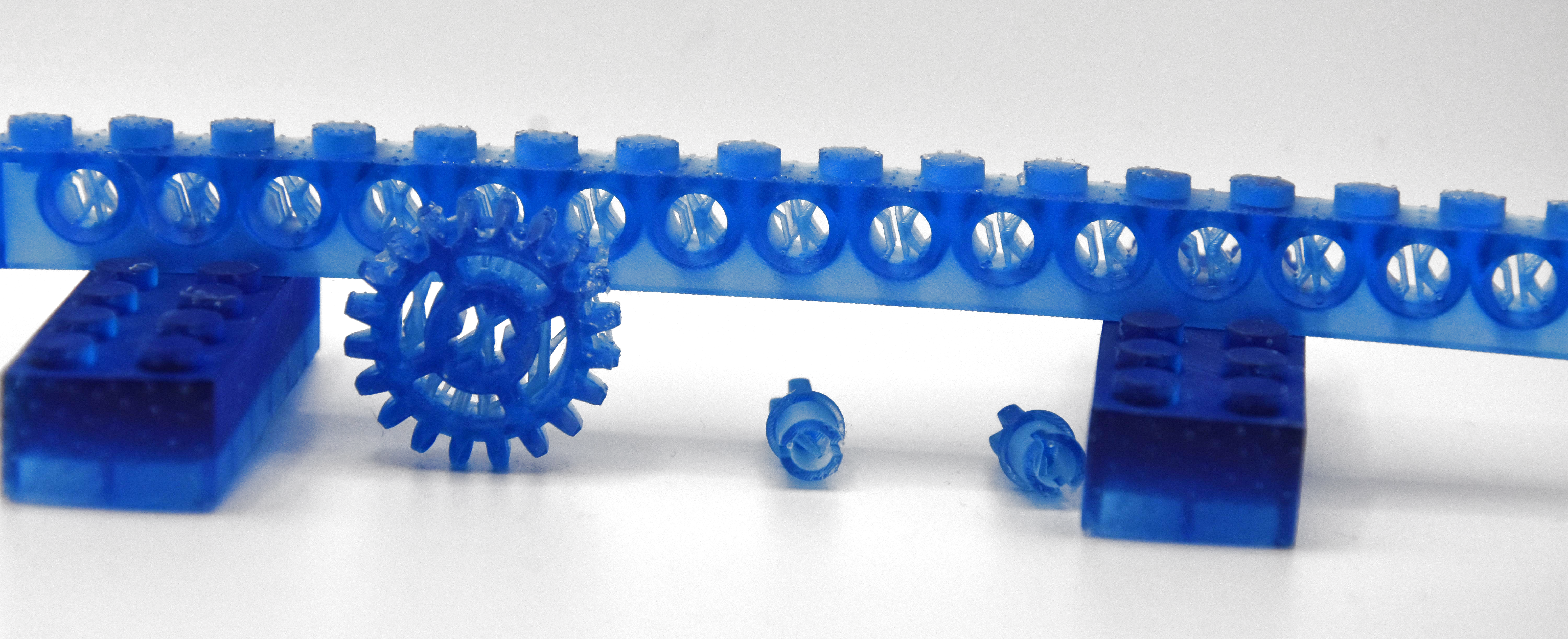
By rotating the figurines to be printed upside-down relative to the build plate this also meant having lots of ugly marks left by the supports, both on the happy buddha and the female knight figurine.
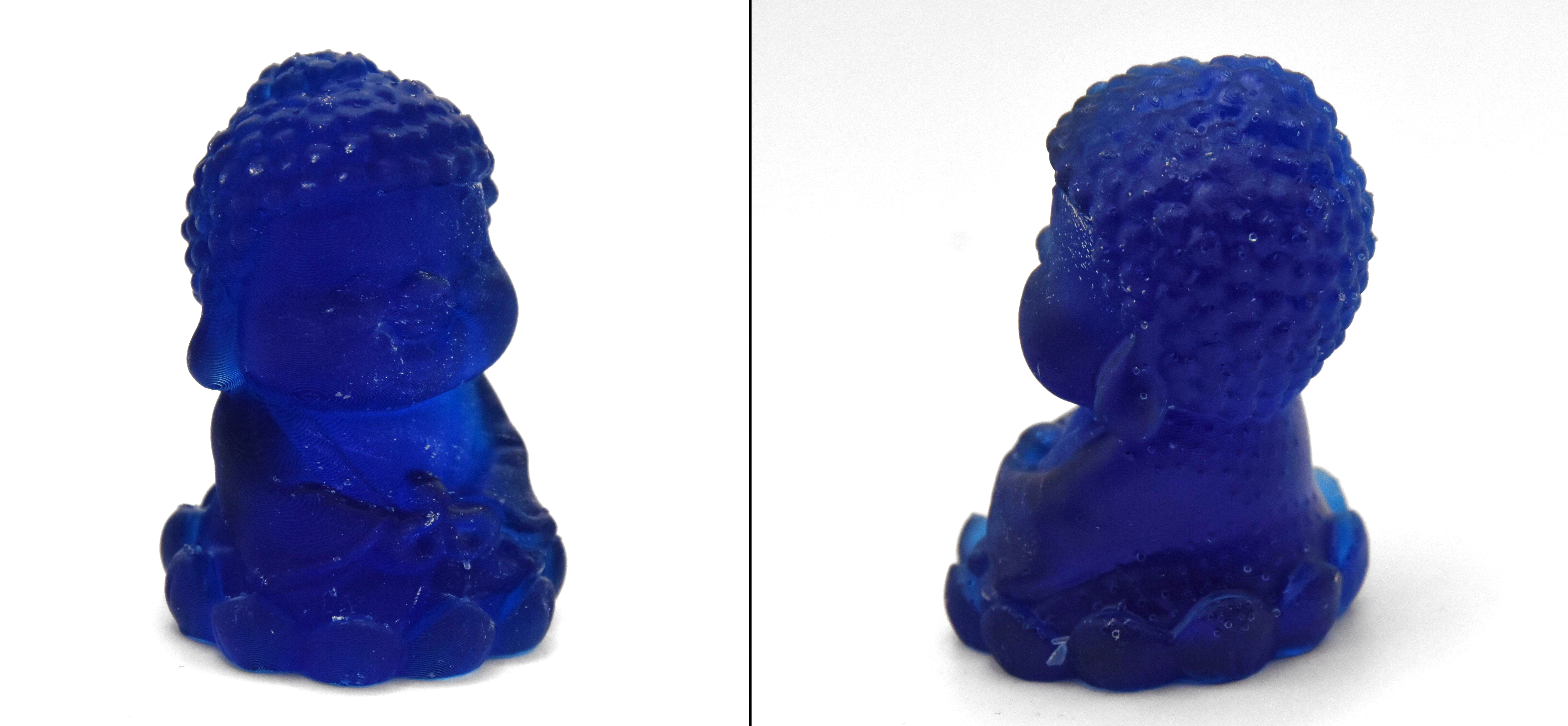
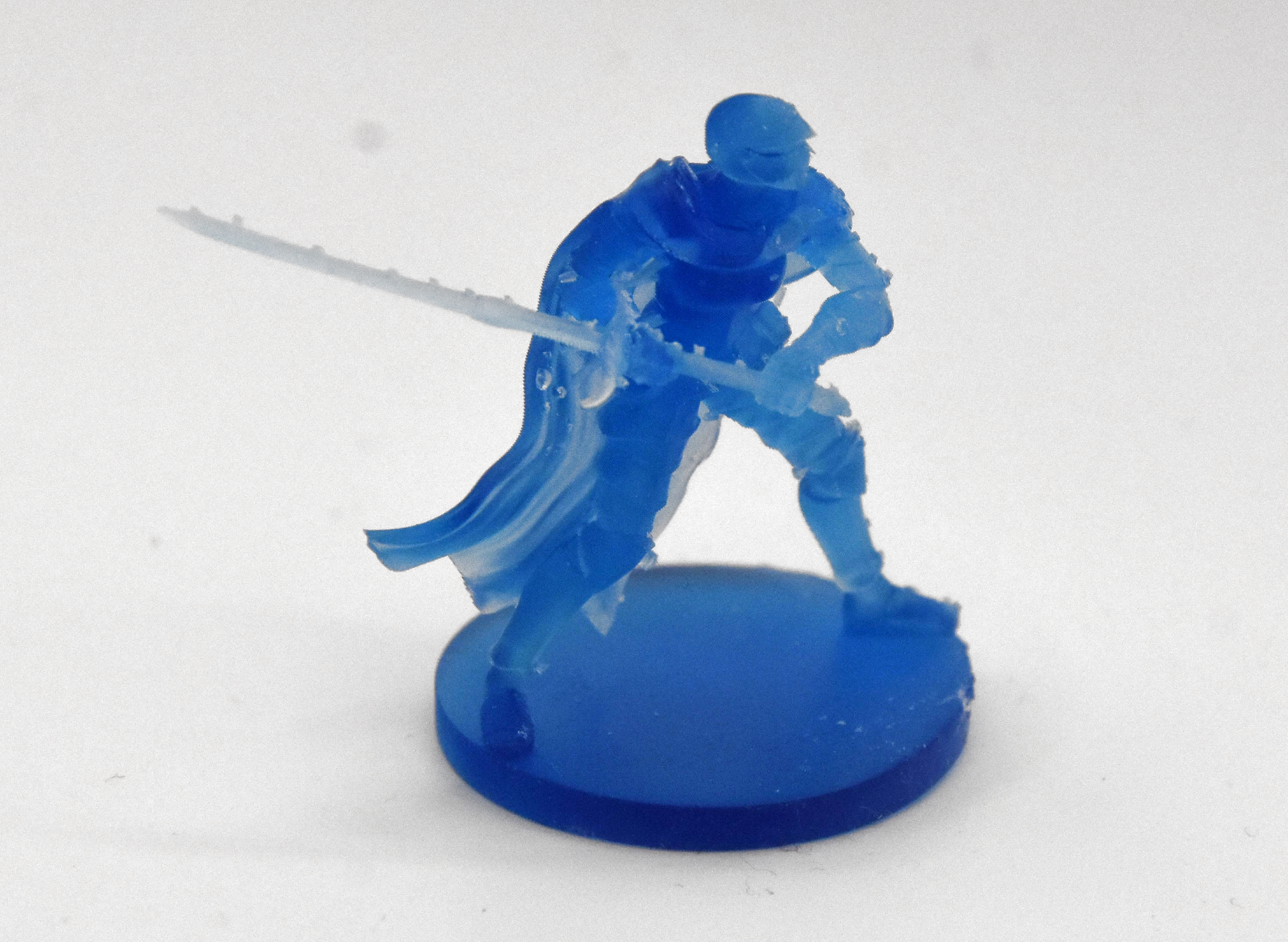
Here the fix seems rather straightforward: angle figurines so that supports contact things like the bottom of a surface where it won’t be as noticeable. Also inspect the auto-generated supports to remove any that are in naughty places and perhaps do some manual supporting if you feel particularly confident.
I did look at a few “how to do supports right” videos and written tutorials, and the general advice seems to be to simply forget about auto-generated supports.
For me an amazing aspect was that both figurines were angled upside-down by the slicer, when everyone prints them with the base towards to the build plate. Exactly how ChituBox’s algorithm here works is a complete mystery to me, but I reckon that this slightly confusing experience may have contributed to the subsequent disaster that occurred with another print.
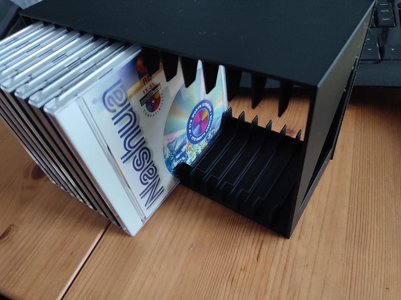
Where things slid sideways and wrapped themselves at high velocity around a phone pole was when trying to print a 16-slot CD rack, specifically this rather nice model by [zenitar3d] from Thingiverse. On an FDM printer this is braindead simple to print: you slap it on the build plate in the slicer, do a sanity check that it physically fits, slice it and let ‘er rip. My only issue here was that OrcaSlicer deemed it necessary to add a brim, so that took some sanding to clean up a razor sharp edge.
On the resin side of things, you enter a torment nexus: you can slap the part on the build plate, but then you risk elephant foot — a thickening at the base where exposure time is longer than for subsequent layers. Even if that’s of no concern, you still need to violently remove the part from the solid metal build plate, which is highly likely to cause damage.
If I still had the LD-002R printer with its flex plate, an aftermarket modification that I had fitted. This would be of no concern with a mere flex-and-pop, but here I’d have to violently wield a metal scraper to convince the build plate and cured layers to part ways. Clearly I need to look into flexible build plates for current SLA printers.
I did try to use the same auto-angle and auto-rotate approach in the slicer, but ChituBox would just always put part of the model outside of the printing area. After a while I grew tired of this and just printed it with the part slightly lifted off the build plate with medium supports like this:
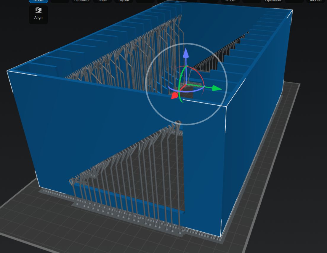
In my defense, I did this in the midst of yet another European heatwave with zero air conditioning, so maybe that had sufficiently fried my remaining brain cells. Regardless, the results were rather predictable.
A little while later I had the good news in the sense that the supports were printing beautifully, but also bad news in that the actual model had been ripped off the supports by the aforementioned peeling forces.
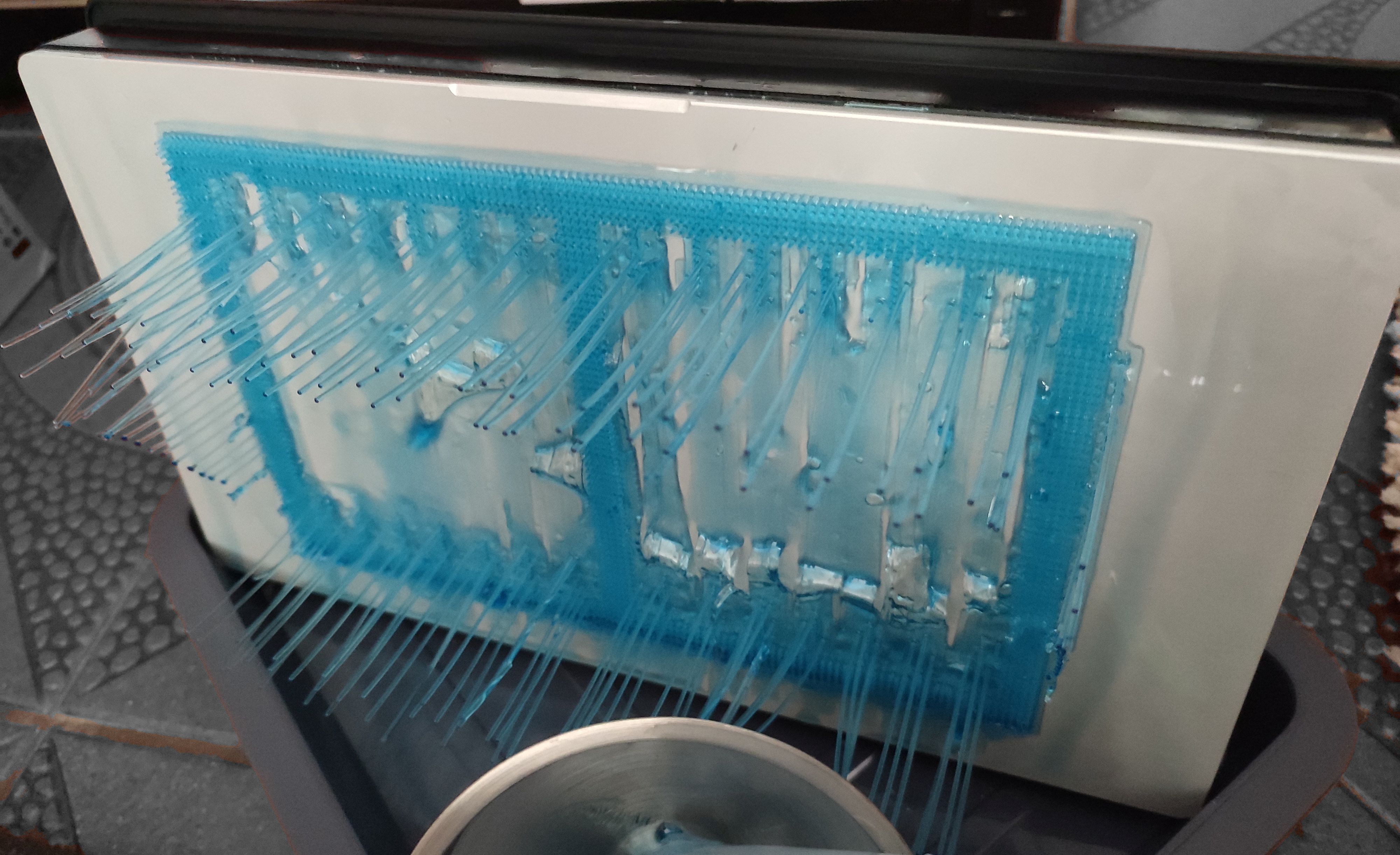
In hindsight this was obvious: the quite solid surface of the model has significantly more surface area than the area contacted by the supports. At the first attempt to peel the newly cured model layer off the nFEP (PFA) film, the tug of war resulted in the supports winning out and the print being a total failure.
You could call this the ‘FDM spaghetti’ equivalent with resin printing, where the FDM’s extruder is printing in empty air, but unlike with FDM printing the subsequent clean-up is less of a sighing, brushing away bits of thermoplastic and trying again with the glue stick, and more of a chemical hazard situation.
Dealing with an SLA resin printing failure sees you draining and filtering the resin from the vat, carefully removing any solid resin from the vat’s film and curing the failed parts so that they can be safely disposed of. All while suited up with gloves, eye protection, and at least a half-face mask with A1P2 filters that still leave you plenty of opportunity to consider whether SLA resin or IPA smells worse when the copious amounts involved of both try to overwhelm the filters.
Where the whole kerfuffle got even worse was when the whole auto-feeding of the resin caught up with me. After ripping the bottle out of the machine I had noticed that the GK3 Ultra had for some reason pulled a vacuum inside the bottle, which could explain some of the issues that I had experienced. This did however also mean that its internal volume had decreased due to the bottle’s deformation.
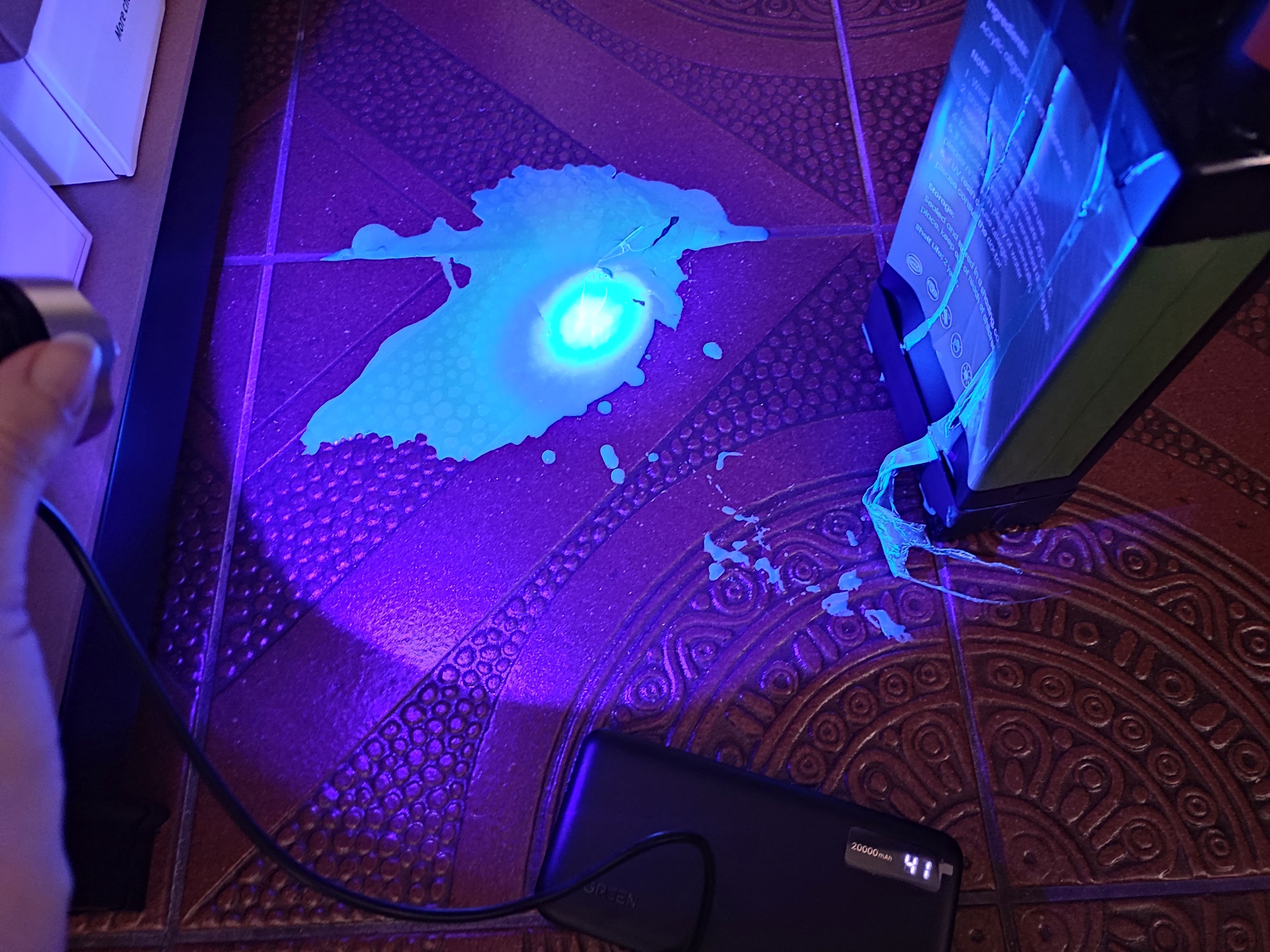
This was a detail that didn’t quite register with me until resin that I was pouring through the filter into the bottle was overflowing onto the floor. Cue copious amounts of colorful cursing and a dash for the paper kitchen towels, followed by a rather illuminating UV exposure session using a handheld UV lamp. Fortunately cured resin doesn’t bond well to tile flooring, so it can be peeled off after curing and tossed into the regular household waste. The pro-tip here is to always use silicone underneath potential resin spills. If only I had done so.
With the floor clean once more, the next challenge was to get the vat cleaned up again. The provided silicone scraper was useful here, but you absolutely need that spray bottle with IPA to soften up the connection between the PFA film and the cured resin.
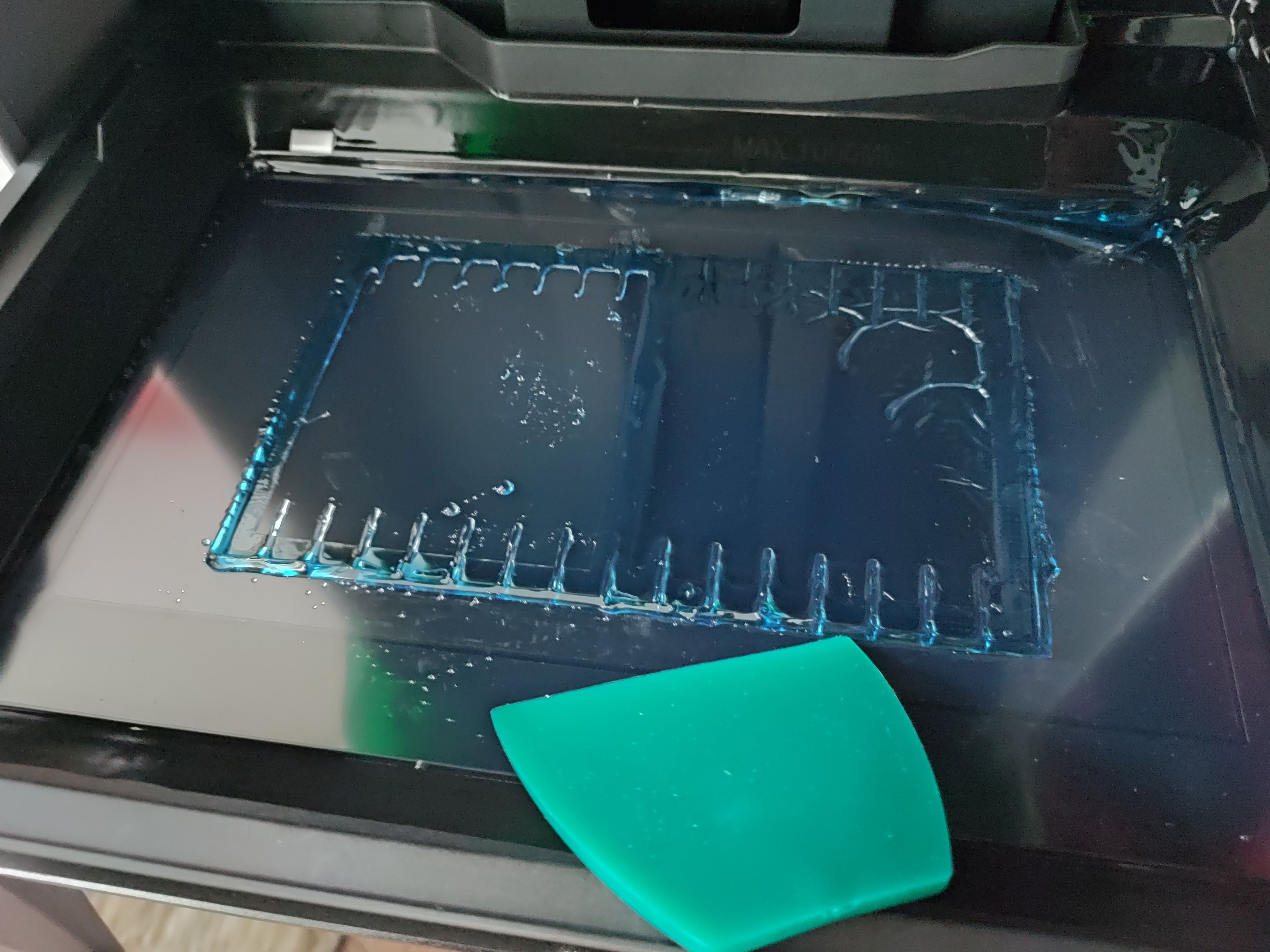
Using the built-in vat curing feature I could cure most of the remaining resin in the vat, but still had to use the handheld lamp to get to corners where it didn’t reach. This is the part that I’m still working on, making sure everything is clean and the PFA film undamaged before I throw myself again at another printing session.
I think the primary lesson that I have learned here is that I still do not comprehend why consumer resin printers insist on having that solid lump of metal that they dare to call a ‘build plate’ — an immovable surface that you have to violently assault with a scraper after printing to make it release printed parts.
After mostly printing with the magnetically attached flex plate on the LD-002R – of course after adjusting its Z-height correspondingly – it still feels like time hasn’t moved at all here.
As a friend of mine remarked when I reported the print failure described in this article, it’s also rather astounding that there’s no simulation of peel forces in slicers to get some idea of whether your supports game is overkill or weak sauce. There are some resin printers that even try to reduce the peel forces by tilting the vat – such as the Prusa SL1S and Form 3 – and there are various ‘tricks’ to reduce the peeling forces, such as lubricating with silicone and PTFE oil, many of which I too have tried with the LD-002R with unclear results, but ultimately you just want to ‘science’ it, as the kids say.
Overall, a resin printing failure isn’t the end of the world, as long as you are mindful of a potential mismatch between the air volume in the target bottle and the resin volume in the vat you’re pouring from. Resin is only nasty until you blast it with UV, when it turns into relatively harmless plastic.
All of that said, I’m still torn on that CD rack model. Theoretically the GK3 Ultra has the build volume for it, surpassing the Neptune 4 in two directions, but it’s not easy to prepare a plate in such a way that the model isn’t ripped off its supports, is not disgraced by a massive elephant’s foot, or worst case the build plate wins and the FEP/PFA film loses the tug of war and rips.
Did I mention rips in the vat’s film? That’s another thing I experienced with the LD-002R back in the day. I was lucky that the resin spill was fairly contained, but I was puzzled for a while why the prints kept failing until I actually drained the vat.
Anyway, after all this learning, it’s time to reorganize and see what I can improve when I next hurl myself at this whole SLA resin printing topic.
Last time we found out the idea of space stations is surprisingly old. By the 1950s, everyone knew we’d be working in beautiful space stations that rotated like a wheel to give us the illusion of gravity. Of course, that didn’t happen. But we did get some practical space stations, even before the current crop. The road to get there, though, was predictably bumpy.
Convair had been studying multi-person orbital stations under Krafft Ehricke since the late 1950s. One result was TASSEL, an acronym for the Three Astronaut Space System Experimental Laboratory. Proposed in 1960, TASSEL was a three-man laboratory intended for an Atlas-Centaur launch into a roughly 200-nautical-mile orbit and missions lasting two or three weeks.
Around the same time, the Air Force asked contractors for proposals for a Military Test Space Station, or MTSS. Convair was one of five companies selected for the study in 1960. The surviving record suggests that Convair’s TASSEL work fed directly into its MTSS proposal.
Then Convair did something unusual for an era overflowing with beautiful paintings of spacecraft that never existed: they built theirs. Well, sort of.
During late 1960 and early 1961, the company constructed a full-scale ground mockup called the Manned Astronomical Research Station, or MARS. The station itself was about ten feet in diameter and fourteen feet high, with two floors for working, cooking, housekeeping, and sanitary facilities. A Mercury-like reentry capsule beneath it brought the whole assembly to about 28 feet tall. You can see a contemporary video about the program below. There’s also a cache of photos and a post by [The Space Review] explaining it all.
MARS obviously wasn’t going to orbit, but that wasn’t the point. Engineers could use it to work on the less photogenic parts of putting people in orbit: life support, oxygen consumption, water regeneration, contaminant monitoring, controls, displays, and simply discovering whether people and equipment actually fit where the drawings said they would. Crews later spent as long as 30 hours inside the mockup.
Exactly where MARS fits among Convair’s various proposals is still being pieced together. Archival evidence indicates that it grew out of TASSEL and closely overlapped Convair’s submission for the Air Force MTSS program. Photographs in the San Diego Air and Space Museum archive are even identified as “MTSS/MARS.” Whatever name was on the proposal of the week, by 1961 Convair had progressed from drawing space stations to building a high-fidelity example on the ground.
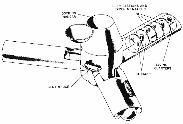
NASA wasn’t far behind. In 1962, Edward Olling at the Manned Spacecraft Center proposed Project Olympus. It would have been an 18-person station intended for launch around 1966 or 1967. It wasn’t the classic doughnut. Instead, three long arms extended from a large central hub, and rotation would provide different artificial-gravity levels at different distances from the center. The station would orbit about 300 nautical miles above Earth.
This is especially interesting because Olympus wasn’t a far-future colony study. It was being considered while Mercury was still flying. Then President Kennedy gave NASA a somewhat more pressing assignment involving the Moon.
Olympus joined the large pile of spacecraft that looked great in presentations.
The U.S. Air Force had another station that got considerably closer to hardware: the Manned Orbiting Laboratory, or MOL. Approved in 1965, MOL would have put two military astronauts into a polar-orbiting station attached to a modified Gemini spacecraft (Gemini B). Its actual classified purpose was high-resolution reconnaissance. You can see some silent footage of some of the hardware in the video below.
They selected astronauts. They built hardware. They modified a Gemini capsule with the unnerving idea of putting a hatch through its heat shield so the crew could crawl into the laboratory behind it. MOL was canceled in 1969 without a crewed station ever flying.
Meanwhile, docking — one of the basic tricks required to make stations useful — was becoming real.
On January 16, 1969, Soyuz 4 and Soyuz 5 docked in orbit. There was no pressurized tunnel connecting them. So Yevgeny Khrunov and Aleksei Yeliseyev put on spacesuits, climbed outside Soyuz 5, traveled across the docked spacecraft, and climbed into Soyuz 4. Two spacecraft had effectively become a tiny space station, but changing rooms required going outside.
Apollo 9 flew less than two months later and provides an interesting parallel. The command module and lunar module could dock, and crews could normally transfer internally. But what if the tunnel couldn’t be used? NASA planned to demonstrate a contingency EVA transfer from the lunar module to the command module.
Rusty Schweickart was supposed to perform the exercise, but space sickness caused NASA to shorten his EVA. He tested the lunar EVA suit and portable life-support backpack from the LM porch while Dave Scott partially exited the command module, but the complete external transfer was never performed.
On April 19, 1971, the Soviet Union launched Salyut 1, the first actual space station. The first crew failed to dock successfully. The second crew, Soyuz 11, spent more than three weeks aboard, but all three cosmonauts died during reentry when their Soyuz depressurized. There is some video from Salyut 1, but no audio.
The Salyut name also concealed a second program. Some of the stations were civilian Salyuts, while others were military Almaz reconnaissance stations similar in purpose to MOL. Salyut 2, 3, and 5 belonged to the Almaz line, although Salyut 2 failed before a crew could arrive.
Later Salyut stations gained a second docking port. That was a huge improvement because Progress cargo ships could bring supplies and fuel while a Soyuz remained attached as the crew’s ride home. Long-duration spaceflight was becoming practical rather than heroic improvisation. Of course, none of them rotated.
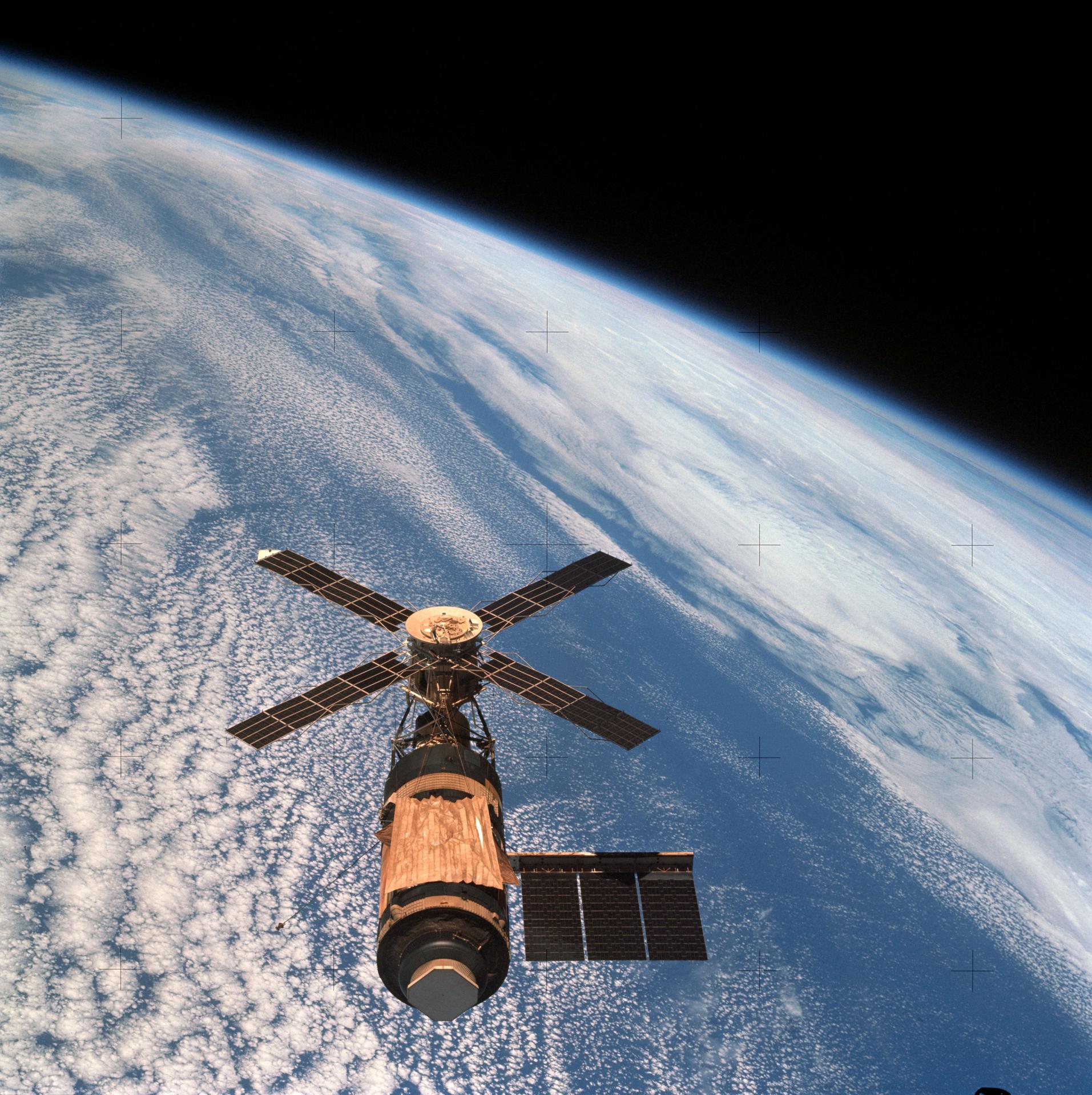
The United States took a different route. Skylab was essentially an enormous converted Saturn V upper stage. Launched in 1973, it gave its crews something previous spacecraft had lacked: room.
Three crews occupied Skylab, staying as long as 84 days. They conducted solar astronomy, Earth observations, medical studies, and experiments designed to determine what happens when human beings spend months rather than days in weightlessness. After all, why build a giant rotating station if people could simply learn to live without gravity?
Then again, we learned that long-term microgravity isn’t free. Bones, muscles, cardiovascular systems, eyes, and assorted other bits of the human body complain when they don’t have proper gravity. Still, a nonrotating station was far easier to build, so rotating wheels stayed on the drawing board.
By the 1980s, NASA was ready to try again. In his 1984 State of the Union address, President Ronald Reagan directed NASA to build a permanently occupied space station within a decade. What eventually became known as Space Station Freedom was supposed to be a large modular facility assembled by the Space Shuttle.
It would support research, Earth observation, satellite servicing, and eventually serve as a staging point for missions beyond Earth orbit.
Freedom went through redesign after redesign as costs and requirements fought each other. It did not rotate. While NASA redesigned Freedom, the Soviets quietly launched something considerably more important.
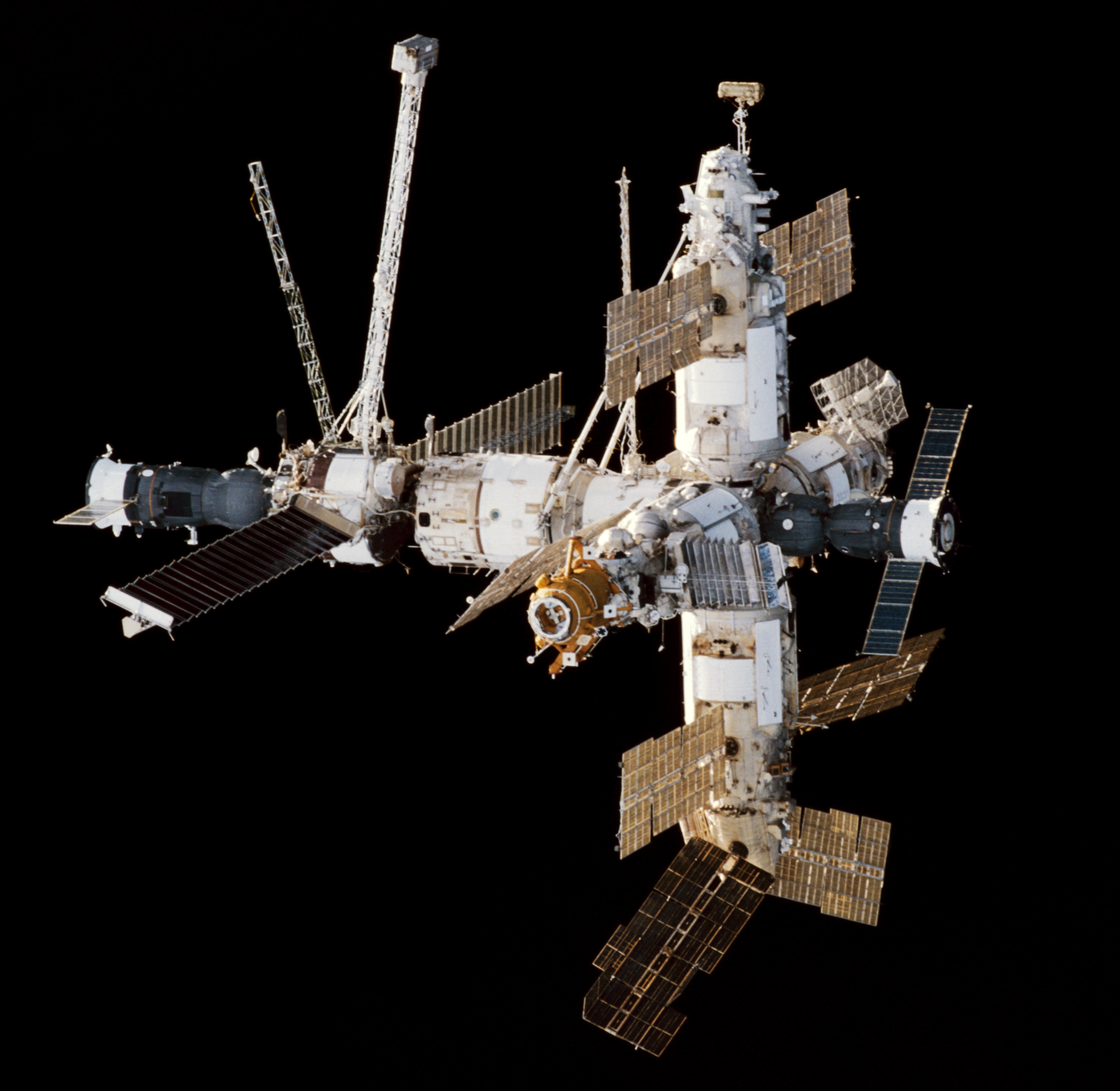
On February 20, 1986, the Soviet Union launched the core module of Mir.
The name means “peace,” although the Russian word can also mean “world.” Unlike the earlier Salyuts, Mir was designed from the beginning as a modular station. Additional laboratory and equipment modules arrived over the years and docked around its core.
It looked nothing like Noordung’s wheel. It looked more like somebody had been assembling an enormous machine in a garage and kept finding useful places to bolt things on.
Mir represented decades of incremental Soviet experience: Soyuz, docking, Salyut, Progress, long-duration crews, orbital repairs, and modular construction. It demonstrated that a space station could become not merely a spacecraft but a place — one that crews could maintain, modify, repair, and inhabit for months at a time.
That may be the most surprising thing about the history of space stations. The rotating station wasn’t some goofy 1950s science-fiction invention. Serious engineers were proposing artificial gravity before anyone had launched anything into orbit. Oberth discussed rotating stations in 1923. Noordung drew a remarkably complete wheel station in 1929. Von Braun made the concept famous in the 1950s. NASA seriously studied rotating stations in the 1960s. The physics works.
We’ve simply never needed artificial gravity badly enough to pay the cost.
If you can tolerate microgravity, a station can be a collection of pressure vessels, trusses, solar arrays, and docking ports. If you insist on one g at a comfortable rotation rate, suddenly you are contemplating a structure hundreds or perhaps thousands of meters across.
Still, Edward Everett Hale put people aboard an artificial moon in 1869. Noordung put them aboard a rotating wheel in 1929. Kubrick had airline passengers walking around one in 1968. So after more than a century and a half of talking about space stations, I have only one question: When do I finally get my rotating space station?
