Normal view

There are new articles available, click to refresh the page.
Yesterday — 22 July 2026Hackaday

The Need for Speed: Internet Speed Measurement (or DIY?)

22 July 2026 at 14:00

Car enthusiasts want to know how quickly they can make a quarter mile. Weightlifters are forever trying to add one more plate to the bar. Internet denizens have their own favorite number to brag about: the result from a speed test.

The ritual is familiar. Close a few browser tabs, click the big “Go” button, and watch the needle climb. Perhaps you pay for gigabit service and see 940 megabits per second, which produces a satisfied nod. Perhaps you see 299 megabits and begin obsessing over network hardware. But before you get too excited either way, try another test. There is a fair chance it will give you a different answer.

That does not necessarily mean one test is lying. “Internet speed” is not a single physical quantity waiting to be measured. A speed test measures the performance of a particular device, over a particular local connection, through a particular ISP route, to a particular server, at a particular time using a particular test method. Change any of those things and the answer can change too.

The Usual Suspects
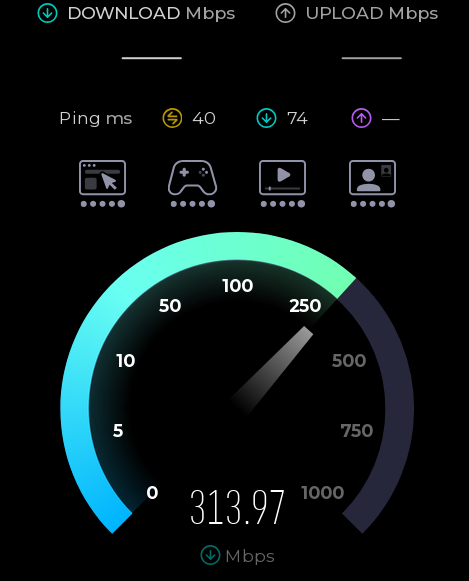
Ookla on a WiFi connection to a 1Gbit Ethernet network. The limiting factor is the 802.11s WiFi link between the computer’s Ethernet port and the router’s.

Speedtest by Ookla is probably the best-known test. It selects a nearby server, although you can choose another. It attempts to saturate the connection with multiple simultaneous transfers. That makes it good at answering the question most consumers are asking: approximately how much aggregate bandwidth can this Internet connection deliver?

Running several connections matters. A single TCP connection must gradually increase its sending rate while reacting to round-trip time, packet loss, receive-window limits, and congestion-control behavior. On a high-bandwidth or high-latency path, one connection may not fill the available pipe. Several parallel connections can ramp up independently and make it easier to reach the link’s aggregate capacity. That number is valid, but it represents something like a busy household, a large segmented download, or several applications operating at once. It does not necessarily predict the speed of one file transfer from one distant server.

Google’s built-in search speed test (search “speed test”) uses Measurement Lab’s Network Diagnostic Tool, or NDT. M-Lab describes NDT as a single-stream measurement of bulk-transport capacity. That makes it an interesting counterpoint to Ookla. A single flow may expose latency, loss, or TCP-window limitations that a multi-stream test can partially conceal. You can also use M-Lab’s own speed test directly.

While you may get similar numbers between the two approaches, you also may not get similar numbers, especially on high-latency connections where Ookla’s multiple streams will help hide latency.

Netflix’s Fast.com is deliberately simple. Open the page, and it immediately begins transferring data from Netflix infrastructure. By default it emphasizes download performance, since its original purpose was to answer a practical question: can this connection deliver Netflix video properly? Selecting “Show more info” adds upload speed and both unloaded and loaded latency.

Fast is barebones and measures speed to Netflix.

The use of Netflix servers is significant. Fast.com measures the route between you and Netflix’s content-delivery network, while Ookla may test against a server operated by your ISP only a few network hops away. A superb Ookla result and a poor Fast.com result do not prove deliberate throttling, but they do tell you that the destinations — or the routes to them — are behaving differently.

Cloudflare offers two related tests. Its Radar Network Quality Test provides a quick summary, while speed.cloudflare.com  gives an extremely detailed breakdown. The latter reports download and upload throughput, idle and loaded latency, jitter, packet loss, server location, and application-oriented quality estimates.
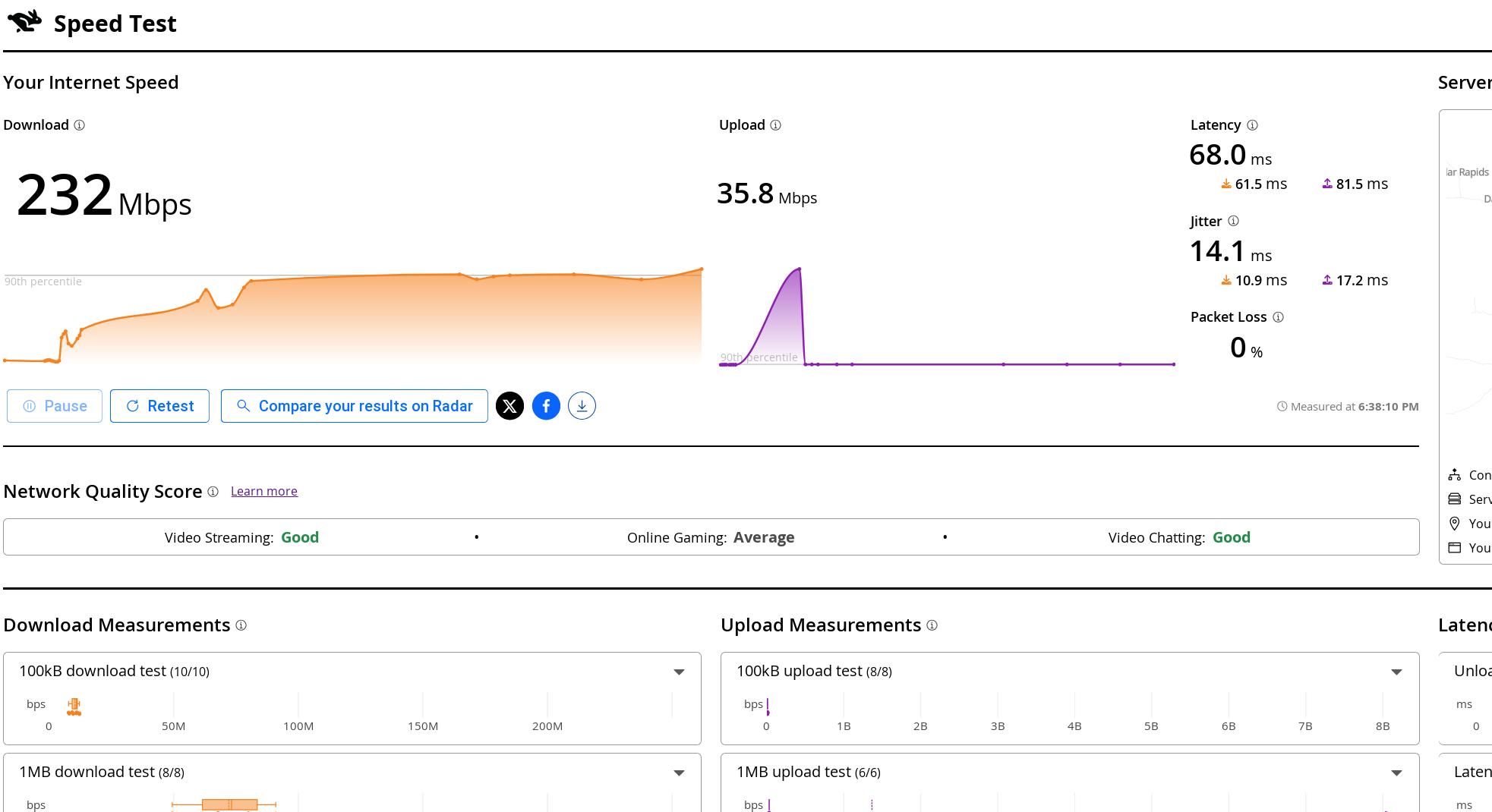
Cloudflare provides a wealth of stats and graphs.

Loaded latency is especially useful. An otherwise fast connection can become miserable when a large upload or download fills an oversized queue in the modem or router. Your idle ping might be 12 milliseconds, but under load it may jump to several hundred milliseconds. That is the classic symptom usually called bufferbloat.

If you want more options, there is testmy.net, which allows you to test upload and download speeds separately, and speedof.me, which keeps a history for you, among others. It isn’t always obvious which ones are measuring a single connection vs multiple ones, so you may have to dig through whatever documentation you can find.

Your WiFi Is Part of the Test

A browser speed test cannot automatically tell you what’s hurting your speed. A laptop connected through marginal WiFi may report 180 megabits per second even though the router has a flawless gigabit Internet connection.

In fact, once incoming Internet service reaches several hundred megabits per second, WiFi is frequently the limiting factor. The link rate displayed by the operating system is not the same thing as usable throughput. Wireless protocols have framing overhead, acknowledgments, contention, retransmissions, and half-duplex operation. The advertised 866, 1200, or 2400 megabit link rate is therefore not a promise that application data will move at that rate.

The numbers printed on WiFi boxes add another layer of optimism. A router sold as “AC1800,” for example, does not provide an 1800-megabit connection to one device. The figure is normally the sum of the maximum advertised PHY rates on separate radios — perhaps 1300 Mb/s on 5 GHz plus 450 Mb/s on 2.4 GHz — with some rounding for marketing. A conventional WiFi client connects to one band at a time, so it cannot combine those rates. The total is better understood as the router’s theoretical aggregate capacity while serving multiple devices across both bands. Even then, protocol overhead, contention, signal quality, and client limitations make actual data throughput considerably lower. Newer WiFi 7 equipment can sometimes combine links using Multi-Link Operation, but that exception does not make the old ACxxxx arithmetic any less misleading.

WiFi also uses shared airtime. Devices on the same channel — including neighboring access points that can hear one another — must contend for opportunities to transmit. A slow or distant client takes longer to send a given amount of data and can consume disproportionate airtime while doing so. Modern access points may provide airtime fairness and other mitigations. One old device does not invariably drag every client down to its rate, but it can still reduce the capacity available to the rest of the network. Interference has a similar effect. A weak signal, a crowded channel, microwave noise, or an overlapping neighboring network causes frames to be delayed or retransmitted. Those retries consume airtime without delivering additional data.

Repeaters and wireless mesh backhaul add another complication. A simple same-channel repeater must receive each packet and then transmit it again over the same shared medium. In the worst case, each repeated hop can roughly halve the available throughput. Modern tri-band mesh systems can avoid much of that penalty by using a dedicated backhaul radio, and Ethernet backhaul avoids it almost entirely.

This means it is entirely reasonable to buy gigabit Internet service and obtain only 300 or 500 megabits per second from a WiFi laptop. Whether that represents a problem depends on the client, radio band, channel width, signal level, backhaul, and local RF environment.

For a meaningful ISP test, begin with a computer connected directly to the router by Ethernet. Stop large transfers and temporarily disable any VPN. Record the chosen server, latency, upload speed, and download speed rather than preserving only the most flattering number. Then run the same tests over WiFi. The difference is an approximate measurement of what the wireless portion of the network is costing you.

Remove the Internet From the Experiment
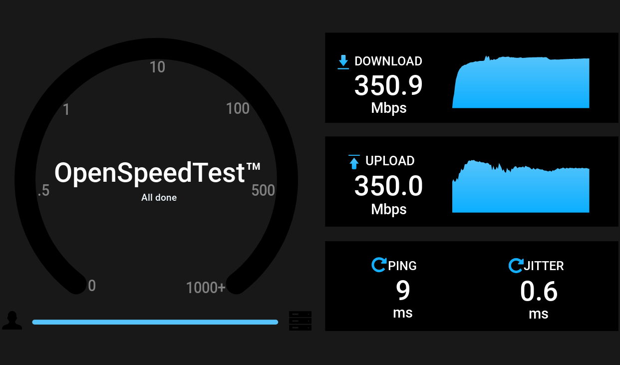
OpenSpeedTest running on an OpenWRT node.

Better still, remove the ISP from the test completely. OpenSpeedTest is a self-hostable, browser-based test. Run its server on a wired computer, NAS, or container, then visit it from laptops, phones, and tablets around the house. Because the traffic remains on your LAN, a slow result points toward WiFi, switching, cabling, or the client rather than the Internet connection.

It is possible to run this on the uhttpd server used with OpenWRT, although you’ll need to coax it to measure upload speeds since the server can’t handle the default method. The trick is to create a CGI script that accepts a large amount of data successfully and then configure uhttpd to run that.

A browser-based local test is convenient, but for serious diagnosis it is hard to beat iperf3, the client/server tool we recently used while testing mesh routers. On one machine (say, 192.168.1.100), start the server:

iperf3 -s

From another machine, run:

iperf3 -c 192.168.1.100

By default, iperf3 uses one TCP connection. Add -P 4 to try four parallel streams, or -R to reverse the direction so that the server sends and the client receives. Those variations can tell you something. If four streams are much faster than one, the network may have enough aggregate capacity but a single TCP flow is being limited by latency, loss, window growth, CPU performance, or offload behavior. If the reverse test is much faster, examine the weaker machine’s transmit path, drivers, antennas, or CPU.

iperf3 can also generate UDP traffic at a specified rate and report packet loss and jitter. That is often more informative for evaluating a wireless link than merely chasing the largest TCP number.

Can Linux Make It Faster?

Linux offers an impressive array of network tuning knobs, which naturally tempts us to turn them. But first, you need to understand what needs tweaking.

Check the negotiated Ethernet rate and interface counters:

ethtool eth0
ip -s link show eth0

A gigabit adapter that has negotiated 100 megabits per second usually has a cabling, connector, or switch-port problem. Increasing TCP buffers will not repair it. Rising interface errors and drops point toward a physical, driver, or congestion problem. TCP retransmits (view with ss -ti) may indicate loss elsewhere on the path.

You can inspect the active queue discipline with:

tc qdisc show

Linux supports queue disciplines such as fq_codel, which combines per-flow queueing with active queue management. It attempts to prevent one large transfer from building an enormous queue and delaying unrelated interactive packets. The kernel documentation specifically lists fq_codel as a sensible queue discipline that works without extensive configuration.

It can be selected as the default for newly created interfaces with:

sudo sysctl -w net.core.default_qdisc=fq_codel

That may improve queueing on traffic leaving the Linux machine. It does not, however, fix a large queue in the cable modem or Internet router. Queue management must be applied at the bottleneck. If the ISP link is limited to 20 megabits upstream, controlling a queue on a gigabit Ethernet interface after it has already handed packets to the router is too late.

For a home connection, the most effective bufferbloat treatment is usually Smart Queue Management on the router. OpenWrt’s SQM system supports both fq_codel and CAKE. CAKE generally provides better performance. However, fq_codel requires less CPU overhead.

High-latency paths introduce a different problem. TCP must keep enough data in flight to fill the bandwidth-delay product. Modern Linux generally autotunes TCP buffers, so the old advice to assign enormous fixed values to tcp_rmem and tcp_wmem is less universally useful than it once was. Before changing them, use ss -ti during a transfer and look for retransmissions, round-trip time, congestion-window size, and whether the receiver window is actually limiting the connection.

Linux also supports selectable TCP congestion-control algorithms:

sysctl net.ipv4.tcp_available_congestion_control
sysctl net.ipv4.tcp_congestion_control

Algorithms such as BBR can improve throughput and queue behavior on some long-distance or lossy paths. But changing the algorithm affects connections sent by that Linux machine; it does not control the remote speed-test server, repair poor WiFi, or eliminate a queue in the router. Congestion-control tuning is therefore a useful experiment for a server, VPN endpoint, or long-haul transfer machine — not a universal solution to slow networking.

Finally, inspect hardware offload features when a Linux system cannot keep up with a fast LAN:

ethtool -k eth0

Advanced network tuning is a bit beyond the scope of this post, but there are plenty of roadmaps down this rabbit hole.

The Lesson

The lesson here is that there is no universally correct speed-test result. Ookla tests how effectively multiple transfers can fill a route to one of its servers. M-Lab examines a single bulk flow. Fast.com tests the path to Netflix. Cloudflare pays unusual attention to latency under load and overall connection quality. OpenSpeedTest and iperf3 can determine whether the Internet connection is even the problem.

Run enough tests, and you will eventually obtain a number worth bragging about. Run the right tests, though, and you may find ways to truly increase real-world performance. If you want to chase that extra 1 kbit per second speed, be our guest — we know how it is. But the truth is that if the Internet is doing what you want it to do, then it is fast enough.


Before yesterdayHackaday

Postal IRCs are Almost a Thing of the Past

21 July 2026 at 13:00

Have you ever found out that something you remember from your youth is now gone, and you didn’t even notice? If you are a certain age, you might feel that way when I deliver the news: You haven’t been able to buy International Reply Coupons (IRCs) at a US Post Office since early 2013. By the end of 2026, you won’t be able to buy them anywhere. The age of the IRC is over.

What’s an IRC?

An IRC from 1978 (public domain).

If that didn’t mean anything to you, you might be too young to remember, or maybe you just weren’t into shortwave listening or ham radio. Although there were other reasons to get IRCs, a radio hobby is the most likely reason a Hackday reader would have bought an IRC.

For radio purposes, here’s the problem. You’ve worked on your station for months, and one winter night, you finally pull in that rare station from Luxembourg. They’ll send you a QSL card to verify that you heard them. You only have to send them a letter telling them what time you heard them, what frequency, and some details about the program you heard. But they probably don’t want to pay the postage required to send hundreds or thousands of cards overseas.

While this is a radio-specific problem, you might find the same issue with pen pals or when trying to buy things from an overseas company.

SASE

If everyone were in the same country, the solution would be easy. Take a stamp, put it on an envelope that has your address on it, and stuff it in with the letter. Or, you could just drop a stamp or two in the letter you sent.

The problem is, US postage won’t help Radio Luxembourg. On the other hand, the effort required for you to buy postage that works in Luxembourg would have been a nightmare.

Enter the UPU

The Universal Postal Union is a UN agency that is effectively an association of post offices in 192 countries. Their charter is to facilitate mailing things worldwide.

The IRCs date back to 1906. The idea is you buy an IRC at your post office. You send it to Radio Luxembourg, or wherever. There, the mail person at the radio station could go to their post office and trade the coupon for enough local postage to send a surface letter worldwide.

Slow Death

A more recent IRC (UPU).

As demand has dwindled, post offices worldwide have quit selling IRCs. As of last year, Australia still did. But Germany, Britain, the United States, and many other countries gave up on them long ago. In fact, Britain’s Royal Mail claimed that the average post office sold less than one IRC per year at the time it threw in the towel.

UPU decided to end IRCs altogether by December 31, 2026. The end of an era and, apparently, not just for radio hobbyists. It is telling that the UPU’s recent editions of IRCs had print runs of 1,000 or even 500. So they obviously weren’t selling very many.

IRCs Other Claim to Fame

If you’ve heard of these before and you aren’t interested in radio, then it might have been in economic history. Have you heard of the Ponzi scheme? It has become a generic term for any business scheme that relies on raising money from new investors to service debt owed to old investors.

However, the original Ponzi scheme dates back to 1920, when Charles Ponzi realized he could buy IRCs in a country where they were cheap and sell them for more in another country. He was happy to accept investors, of course.

The problem is that profits are thin, and the costs of acquiring and transporting large numbers of IRCs quickly swamp most potential profits. Fluctuations in currency exchange rates take the rest.

Goodbye!

So the end of the IRC marks a closed chapter for ham radio and swindling. There were probably other uses, too, that are now consumed by electronic mail, payment systems, and the like.

You have to wonder what adventures IRCs went on during their global travels. The video below shows one’s story.

Launching Rockets is Hard, Bring them Back is Harder

By: Tom Nardi
20 July 2026 at 10:00

Since the first V2 rocket sailed above the Kármán line back in 1944 and right up until the modern era, the trajectory of most space-bound rockets was more or less the same: after expending their propellants they would either crash into some desolate steppe or plunge into the ocean. In either event, the rocket was disposable. The important bit up top might go on to explore the stars or send a human crew off on their mission, but the booster rocket that lifted the spacecraft out of the atmosphere was always going to be sacrificed for the cause.

But in the 1970s NASA had a wild idea: what if we didn’t smash a brand-new rocket valued at millions of dollars into the ocean every time we wanted to put something in orbit? Instead, they would build a hybrid space vehicle that blended the vertical takeoff and raw power of a rocket with the capabilities of an airplane, allowing it and whatever it was carrying to make a gentle runway landing at the end of its mission. As such, the Space Shuttle was born.

With the benefit of hindsight, we now know the Shuttle wasn’t quite the spaceflight revolution that NASA had hoped for. The age of reusable rockets didn’t truly begin until 2015, when SpaceX landed the first stage of their Falcon 9. To date they’ve repeated the feat nearly 600 times, all the while increasing the reliability and speed of their operations. Today the Falcon 9 is the most prolific launch vehicle in history, and nearly every other rocket in active development is being designed to include some element of reusability.

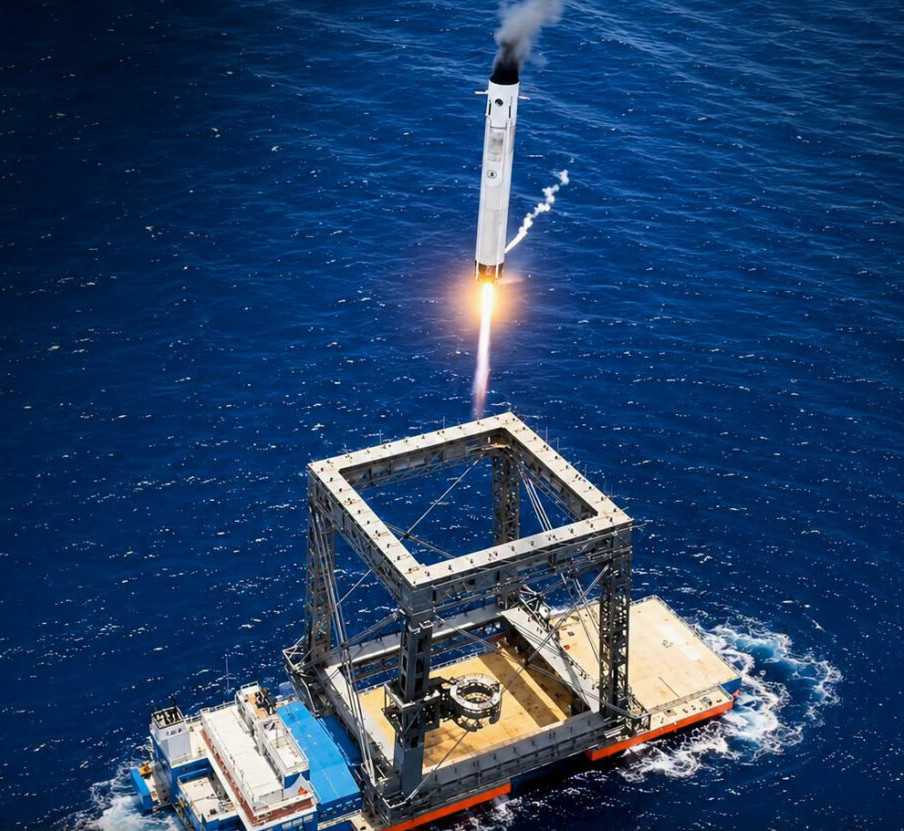
Most recently, China demonstrated that they could recover their Long March 10B rocket by gently bringing it down into what amounts to a giant butterfly net. While it might seem a bit quaint compared to rockets that land on their tails like something out of a 1950s sci-fi movie, the idea offers considerable promise.

There and Back Again

But why did it take 70+ years before we were able to regularly refly orbital-class rockets? It’s not that there’s anything inherently complex about reusing a spent rocket. Sure, there’s a case to be made that material science improvements have made the engines robust enough for repeated use. But even if you had to rebuild the engines after each flight it would still be better than slamming the whole vehicle into the ocean. Similarly, there’s nothing particularly unique about the structure of the Falcon 9 that enables it to fly multiple times — it’s a big metal tube with tanks inside of it, just like essentially every rocket that has flown before it.

The revolutionary technology demonstrated by SpaceX in 2015 didn’t have anything to do with making their rocket go up, it was that they were able to safely bring it back without damaging or physically altering it. The Falcon 9 first stage that came back to Earth was in the same condition it was when it left the launch pad eight minutes or so earlier, albeit with empty propellant tanks and a layer of soot on the outside.

As such, most of the variability we see when comparing the reuse of past, present, and future rockets comes not from how the vehicle ascends, but how it ultimately comes to rest back down on Earth.

Splashdown is Easy, But Rough

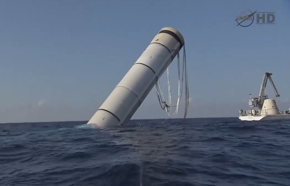
Without question, the easiest way to recover a rocket intact is to simply slow it down before it hits the surface of the ocean using parachutes This is how all American crewed capsules, and more applicably the Space Shuttle’s Solid Rocket Boosters (SRBs), have been recovered after their flights.

Once pumped out, the hollow SRBs could be towed to shore.

But even when descending under multiple huge parachutes, splashdown isn’t exactly a gentle event. It could probably best be described as “survivable”, in that the vehicle and crew will come through the experience in one piece, but neither is likely to be terribly happy about it.

The situation of course ends up being even worse for the rocket, as its structure is going to be subjected to the brunt of the impact force. Additionally, a complex aerospace vehicle getting partially submerged in salt water is a recipe for corrosion and electrical issues, to say nothing of the thermal shock the hot engines will experience when getting dunked.

One could argue that the only reason this method of recovery worked for the Shuttle SRBs is because of their relative simplicity when compared to a liquid-fueled rocket capable of independent flight. At the risk of oversimplifying the structure of the SRB, at splashdown it was effectively a hollow tube with minimal avionics and thrust vector control (TVC) hardware that could simply be replaced before the next flight.

Still, the NASA document Solid Rocket Booster (SRB) Refurbishment Practices goes over the considerable work required to bring each booster back to flight status after coming down in the ocean. Given the challenges of refurbishing the boosters, it’s perhaps unsurprising that NASA elected to forgo their reuse on the Space Launch System despite its SRBs being largely identical to their Shuttle predecessors.

Teaching Rockets New Tricks

In the very early days, while they were still trying to reach orbit with the Falcon 1, SpaceX had actually considered a Shuttle SRB-style recovery procedure. But in the end they decided to outfit the Falcon 9 with deployable landing legs and the rest, as they say, is history.

The DC-X demonstrated propulsive landing in 1993, but couldn’t reach orbit.

Landing legs allow a rocket to come down on effectively any flat surface, be it a concrete pad next to the launch facility or a floating platform. But there are some fairly serious drawbacks to this approach. For one thing, the requirement for precise terminal guidance means parachutes are out of the question. The rocket needs fins, attitude thrusters, or other control surfaces to come down on the center of the pad.

It also means the rocket needs to perform a propulsive landing. That is, use its own primary engines to bring its velocity on touchdown to as close to zero as possible. This in turn requires engines that can not only restart in flight — a capability that has not traditionally been required by first stage boosters — but are able to throttle down low enough to control the rocket’s descent without simply pushing it back upwards. It’s difficult to overstate how unnatural a state of operation this is for a rocket. Indeed, it’s the antithesis of how nearly every rocket has operated since the Song Dynasty started experimenting with gunpowder in the 10th century.

Even if you can accomplish all that, the true cost of landing a rocket is in the extra mass. Although the legs will be stowed away and unused for 99.8% of the rocket’s flight time, it still has to lug all that weight uphill. If that wasn’t bad enough, there’s also the extra weight of whatever control mechanism is in place to guide the rocket’s descent trajectory as well as the propellant that needs to be kept in reserve for the landing burn.

All told, landing a rocket on legs comes with a massive payload penalty. In the case of the Falcon 9, the rocket’s maximum capacity to Low Earth Orbit (LEO) in its expendable configuration is approximately 22,800 kg (50,300 lb). But when outfitted with the hardware necessary to land, that number is reduced by nearly 25% to 17,500 kg (38,600 lb).

Dropping the Dead Weight

There was a time, not so very long ago, when critics doubted the financial viability of recovering and reusing rockets like the Falcon 9. But today, reuse has gone from theoretical to standard operating procedure. Outside of a few Old Space holdouts, it’s top of mind for every launch provider and critical for remaining competitive in a fast-moving commercial market. In November, Blue Origin even managed to land their New Glenn heavy-lift rocket on only its second flight.

So at this point the question isn’t whether or not future rockets will be reusable, but rather, what is the most efficient way to achieve that reusability?

The first stage of Starship after being caught in mid-air.

With that in mind, it’s easy to see the appeal of China’s net recovery. While the rocket must still perform a propulsive descent — although in theory the necessary positional accuracy, and therefore the technical challenge, is somewhat reduced — it doesn’t need to have landing legs installed. This mass savings increases the vehicle’s useful payload capacity, which in turn makes it more profitable to operate. Achieving the same end goal while being easier and cheaper is an improvement in anyone’s book.

Admittedly, having the rocket come down in a huge net adds a certain amount of whimsy to the whole endeavor, but the overall logic is sound enough. It should also be said that SpaceX, for all the success they’ve had with landing their Falcon 9 on a set of deployable legs, are themselves planning on catching both the first and second stages of their next-generation Starship vehicle. Instead of a net, their goal is to pluck the rocket out of the air with a huge robotic pincer mechanism.

One is reminded of the old joke about how the Americans and Russians approached the problem of writing in space: NASA spent millions of dollars developing a pen that would work in microgravity, while their Russian counterparts simply used pencils. If China can demonstrate the ability to reuse a rocket they snagged in their net, the more elaborate methods of recovery employed by American rockets may one day look like a similarly overengineered solution.

Putting Some Zig in a Linux-Based 3D Printer

15 July 2026 at 10:00

Having Linux on so many devices is both a blessing and a curse. Sure, it is great that you can hack on things and modify them or even totally repurpose them. But it also means you have a fleet of Linux devices you have to manage and keep track of.

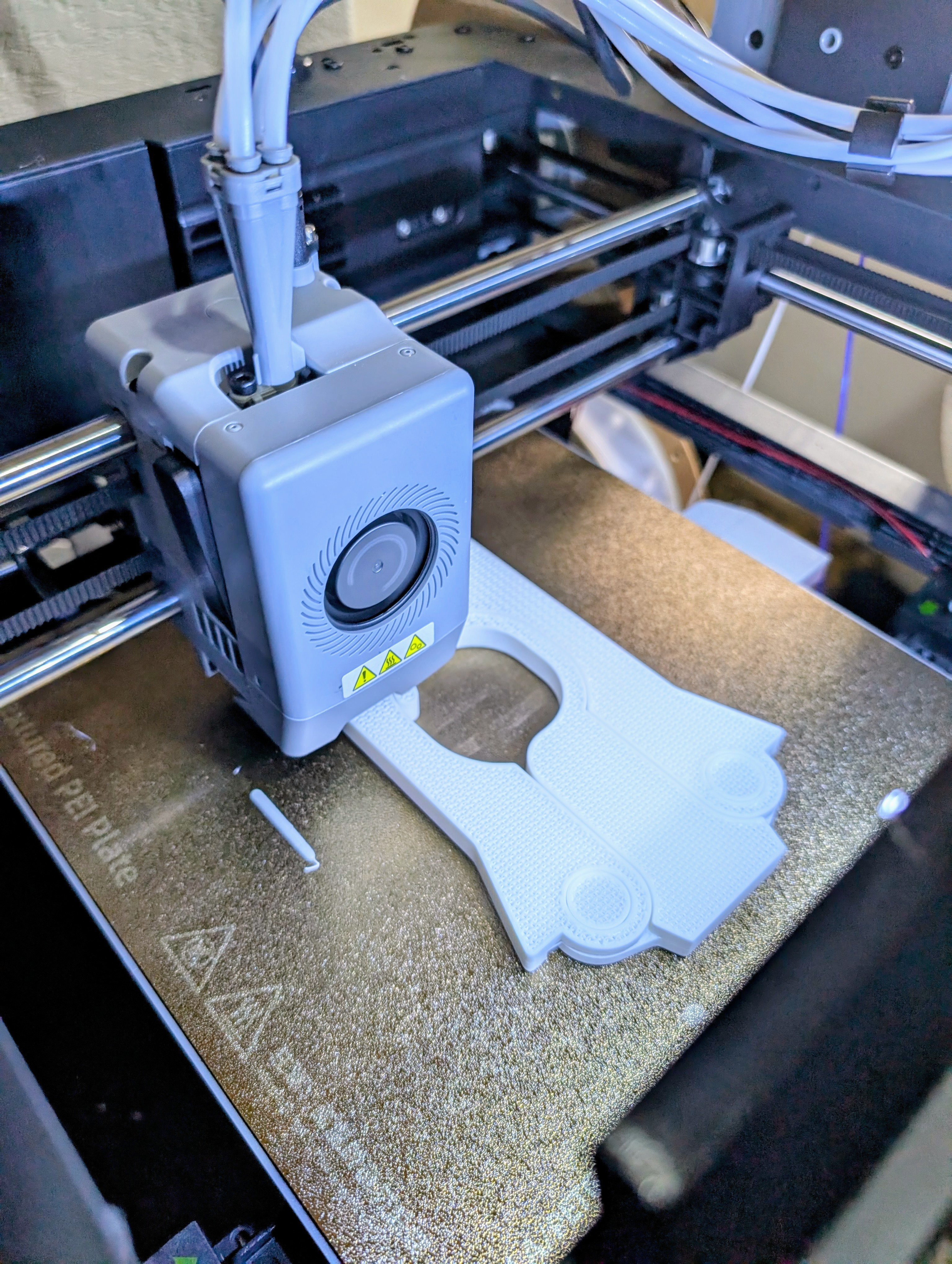
My current “main” 3D printer is a Flashforge AD5X: a nice, cheap machine that does four colors with the purge/exchange method. It sort of runs Klipper. I say sort of because Flashforge has Klipper running on a Linux host in the box, but it is massively crippled and modified. I’m sure it works for most folks. I’m also sure that if you know nothing about Linux, Klipper, or 3D printing, the experience is probably better thanks to all the cloud point-and-click interfaces. But, of course, I check none of those boxes.

I’ve had the printer for probably a year or more. Almost immediately, I put a “mod” on the printer to give it a more true Klipper interface and gave me things like shell access. There are several that I think will do this, but I used Zmod, which doesn’t totally replace the printer’s firmware; it just sort of patches it and extends it. You can easily bypass or even remove it and go back to the stock printer, although I would not want to.

In my case, the issue was a printer, but the same idea might apply to any embedded Linux system, from a router to a thermostat. Sure, it runs Linux, but is it Linux you can change?

The Problem

The AD5X runs Linux… sort of.

The Flashforge firmware and Zmod both will run on the AD5X’s little sister, the AD5M. However, the AD5M has a significantly less capable processor board than the AD5X. That means that Linux on the boxes is very stripped down. From Flashforge’s point of view, no one should be in the Linux OS anyway, and the author of Zmod probably figures every byte used is a byte taken away from the user or other advanced Zmod features.

It may seem like a first-world problem, but there were two things that irked me about the printer’s Linux. There was no less or more command for poking around files. There was also only vi as an editor. I did a few hacks to make myself happy. I wrote a pager in shell script, for example. I would try to remember to use my desktop emacs and tramp to edit files on the box. But it was a shame that there were some very basic tools lacking. Besides that, even the tools that were there like ls lacked help commands in case you want some strange option you can’t remember.

No Install

To save space, the printer doesn’t really have programs like ls, cat, and grep. Instead, it has a single busybox executable. This is common on small systems. You get one copy of the libraries and a single executable that will do all the work you need. You can invoke, for example, grep by running “busybox grep” or, if you make a symlink to busybox named grep, the user may never realize that you don’t really have grep installed.

However, busybox has to be built. You can’t easily install packages to it. So I could just run some package manager and install less or anything else. My plan was to produce a new busybox package myself to supply at least the missing commands and maybe some of the more basic ones, too. How hard could it be?

How Hard, Indeed

The first issue was figuring out exactly what the printer was running. The OS was a buildroot compile as shown by /etc/os-release:

NAME=Buildroot
VERSION=2020.02.1-g0b1f992-dirty
ID=buildroot
VERSION_ID=2020.02.1
PRETTY_NAME="Buildroot 2020.02.1"

In theory, you could probably try to rebuild everything from that information, but it seemed like a bad idea. Who knows what changes they’ve made or what strange dependencies were out there?

The next piece of the puzzle was the architecture. It turned out to be MIPS, which has many variations, a problem that would come back to haunt me later. To figure it all out, I grabbed busybox from the machine and copied it to my regular computer. This let me read the elf file:

# readelf -h busybox
ELF Header:
Magic:   7f 45 4c 46 01 01 01 00 03 00 00 00 00 00 00 00
Class:                             ELF32
Data:                              2's complement, little endian
Version:                           1 (current)
OS/ABI:                            UNIX - System V
ABI Version:                       3
Type:                              EXEC (Executable file)
Machine:                           MIPS R3000
Version:                           0x1
Entry point address:               0x403fa0
Start of program headers:          52 (bytes into file)
Start of section headers:          775880 (bytes into file)
Flags:                             0x70001405, noreorder, cpic, nan2008, o32, mips32r2
Size of this header:               52 (bytes)
Size of program headers:           32 (bytes)
Number of program headers:         10
Size of section headers:           40 (bytes)
Number of section headers:         30
Section header string table index: 29

Forensics

Just knowing that the CPU was MIPS was hardly enough. Note that the processor could have been big endian, but this one was little endian. What’s more, the flags show a few things, and the important ones would turn out to be mips32r2, which defines a particular set of instructions, and nan2008, which means everything is using a more modern floating point stack compared to some older MIPS setups.

The next step is to find a toolchain that can run on my Linux box and produce executables for such a machine. There were two main candidates that I thought about: zig and crosstool-ng.

Zig

You may remember that Zig is a completely different language from C. So it might not make sense that I want to compile busybox, a C program with Zig. However, Zig has an interesting feature. It can pretend to be gcc, and maybe compilers for some other languages too. The idea is that if you have a lot of C code, you could start changing over to Zig without having to convert everything today or even ever. Using CLang and LLVM, Zig purports to be able to just drop in a project as the system C compiler.

So why does that matter for this project? Zig also supports a lot of targets, including MIPS, and provides run time libraries for them. So if I just tell the build system to use Zig, everything will be fine, right?

Right…

Naturally, this didn’t work as well as I expected. It could be that I don’t understand Zig well enough, but passing --target mipsel-linux-musleabihf -mcpu=mips32r2 to zig cc couldn’t produce a working ‘hello world’ program. The reason? Zig appears not to supply a nan2008 library for MIPS. Or maybe I just didn’t know how to enable it. As far as I can tell, Zig might have done the right thing for mips32r6, but that, unsurprisingly, led to illegal instruction problems. Besides, I wanted to stick as close to the existing setup as possible.

I could have made Zig rebuild its libraries, but then I might as well build a full toolchain. However, I wondered if floating point would matter much for what I was doing, so I decided to cheat. I let Zig build an executable, and then I simply patched the output header to say it used nan2008. It worked for a simple program.

Busybox

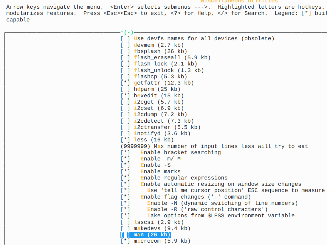
The configuration menu for busybox lets you customize it to your liking or, at least, requirements.

Configuring busybox is a matter of using a menuconfig system similar to building a kernel. I mainly asked it to make a static copy in options and then just picked a bunch of things I wanted, especially less and more.

Many programs, including less, have options to help you minimize the size. For example, you could disable regular expressions or make it not read $LESS for options. I left nearly everything on for most of the programs.

Once it was ready to go, I needed to run make with the Zig compilers and then do the patch to fool the printer into running it.

The command line that worked the best turned out to be: make V=1 CC="zig cc -target mipsel-linux-musleabihf -mcpu=mips32r2 -static -Os" STRIP='llvm-strip' -j6

Of course, you could adjust the -j6 to suit how many CPUs you have. I like to use about 1/2 of mine when compiling. Then the patch is as simple as:

printf '\024' | dd of=busybox bs=1 seek=37 count=1 conv=notrunc

Did it Work?

Once I transferred the file, renamed to busybox-ad5x, over to the printer, I was able to successfully run things like busybox less or even busybox ls. Everything seemed to work. You can ask busybox to install a bunch of symlinks for everything it knows how to do, but I wanted to start small, so I only made symlinks for things that didn’t already exist in the native busybox.

Once I didn’t find problems, I eventually replaced even the old busybox utilities with the new ones. I even made busybox-ad5x a symlink and renamed this version as busybox-zig because I wanted to try one more experiment: using crosstool-ng to make a proper toolchain.

Next Time

But that’s a whole other topic for another day. For now, Zig — with a little patching — got the job done. There are many ways to get things done under Linux. Turns out it is very hard for a vendor to totally lock down a system, and if there is a way in, then there is almost always some way to tune things to your liking. Busybox is a great tool for stripped-down systems. Even floppy-based boots.

UDP Broadcasting and the Joys of IPv4 Subnetting

14 July 2026 at 10:00

In the previous installment on UDP broadcasting and service discovery, the basics of both were explored, including an implementation in the form of NyanSD and its protocol. Contained in the comment section was a very good demonstration of why one of the most exciting aspects of software development is the opportunity to share your latest creations with other people. This being the ability to get solid feedback on all the points – including any potential boneheaded omissions – that you really should address, whether intentional or accidental.

The most pertinent point raised was definitely that of broadcast addresses and IPv4 subnets, with the latter topic especially being something that the sysadmins at the office would talk about all the time, but which us software developers were always happy to ignore as something that didn’t concern us. Turns out the joke was on me and everyone else – like our esteemed readers – who thought that they could escape the fascinating world of subnets, as today we’ll take an in-depth look at what subnets are and how they are relevant to the world of UDP network discovery.

I somewhat alluded in the first article to the topic of ‘which broadcast address to use’ as being somewhat of a rough topic to figure out, which is clearly why I just stuck to a blatantly ‘works for me’ /24 subnet that usually will work on networks, until it does not.

Subnet And Conquer

Basic subnetting concept. (Credit: Michel Bakni, Wikimedia)

The short version of ‘what is a subnet’ is to point at the subnet mask that we have been mostly mindlessly mashing into networking configuration dialogs along with the IPv4 address for many decades now. Usually this takes the form of 255.255.255.0, which is just the human-readable version of the actual bitmask. Here the loopback interface already tends to use 255.0.0.0 as its netmask, which is a detail that tends to be easy to gloss over as this is just one of those local OS things.

Putting netmasks in the crudest and simplest terms, they are a bitmask that is used to identify how an IPv4 pool of addresses is split up by defining which bits of the 32-bit IPv4 address identify a subnet. Normally we call the trailing part of an IPv4 address (the .123) the host identifier, with the preceding section the network identifier.

By masking part of this host ID and using it to create a subnet identifier, we can then use this for additional routing, just at the cost of a reduced number of possible host IDs within that subnet.

As an example, the common 255.255.255.0 mask identifies the first 24 bits (3 bytes) of the 32-bit (4-byte) IPv4 address, hence the mask being referred to as /24. With this mask, the remaining host ID bits allow for 256 hosts, of which two are not used for hosts: the first (e.g. 192.168.0.0) and last (e.g. 192.168.0.255) in the range. The last host ID in the range forms the broadcast address for that subnet.

This is why, for a /24 subnet, you can generally get away with just slapping a .255 on the end of an interface’s address, but also why for other subnet configurations it’s likely to explode violently.

To get briefly back to the loopback’s /8 style netmask, this means a single subnet with a maximum of 16,777,214 hosts, which ought to be sufficient for local system networking shenanigans. Its opposite extreme would be the /31 style netmask, which with just two potential host IDs is practically useless.

IPv6 subnetting is similar, but due to the much larger address pool and differences in the protocol this is a whole other kettle of fish that is as likely to send a network administrator’s heart racing in excitement as it is to make the average software developer run away screaming. This can be a fun topic for another day, perhaps.

This overview of IPv4 subnetting also skips over details like the different classes of IPv4 subnets beyond the Class A type here, but those are happily left to sysadmins and kin for now.

Sub-casting

In order to thus obtain the broadcast address for a given network interface you need to know two things: the IPv4 address and its associated netmask. From this you can then tell three things: the subnet ID, the broadcast address in that subnet, and the current host ID. Of these we only really care about the the second item.

Although you can obtain the broadcast address yourself by applying the netmask to the address, the OS’s APIs tend to happily give you the precomputed broadcast address. If that’s not your style or not an option, a manual procedure is to:

  1. Determine the number of host ID bits using the netmask.
  2. Set all bits to 1 in these bits to get the highest possible host ID.
  3. Use this value along with the original masked (i.e. network ID) bits to obtain the broadcast address.

If we thus start with a 192.168.0.0/24 network, we end up with 192.168.0.255, while for a 192.168.0.0/26 network with just six bits available the maximum value is 64, ergo we get 192.168.0.63, since we start counting at 0.

With this we can now broadcast UDP packets on any interface without any (major) worries.

Local Broadcast Address

A small glitch in the whole above story is that there’s actually another broadcast address, one which is always the same for each interface and can be considered to make the whole preceding explanation completely irrelevant. This being the local, or limited, broadcast address, which is either the best thing since sliced bread or the worst sin ever committed in the history of IP networking, depending on whom you ask.

This cheat code takes the form of the address 255.255.255.255 and if you send a packet on a UDP socket to it, you’ll get happy UDP responses from any service that is listening on the specified port. This raises the point of why you’d not just use this broadcast address on all interface, rather than bother with all the earlier described nonsense.

The only major difference between this local broadcast address and the earlier described directed broadcast address is that the latter can also be used to target a foreign network, instead of just the local network. This makes it a very attractive option if you just want to query the local network with UDP broadcast packets.

As for why you’d not want to use a local broadcast address, I couldn’t really find any references or citations on why this would be the case. Both would appear to be perfectly valid approaches to broadcasting, each with its own pros and cons.

Bugs

One final topic was my mistaken hardcoding of a /24 style broadcast address in NyanSD. Here reader ziew helpfully pointed me towards the Poco::Net::NetworkInterface::broadcastAddress() function, which seemed perfect. Unfortunately Poco’s implementation at least on Windows 10 appears to be rather broken.

After getting only 0.0.0.0 as broadcast address from this function, I had a bit of a look at what was happening, including checking what I got as subnet mask both for the default index parameter and for the next index. Across two different Windows 10 installations and both GCC in MSYS2 as well as MSVC 2017/2022 with various versions of Poco the returned values were… interesting enough to file a bug report on the Poco issue tracker.

Clearly this isn’t going to be fixed just yet, but on the bright side the horrific atrocity that I committed by hardcoding a /24 broadcast address will still work on basically every home LAN out there that NymphCast is likely to be used on.

Maybe I could just switch to a local broadcast address and that’d be even better. Feel free to torch down this idea in the comments, just be sure to provide solid reasoning and cite your sources.

A Complex Topic

Writing out the above pretty much clarifies I think why past me got a bit overwhelmed when trying to ‘just do a UDP broadcast thing’. Even just scratching the surface of IPv4 subnets and not even venturing into IPv6 territory makes one already feel a bit antsy.

Certainly, one could totally argue that anything other than a /24 network is unlikely to be encountered outside of certain government and business networks with either very specific needs, very enthusiastic sysadmins, or both, but it’s always better to design software with such real-life scenarios in mind.

A Brief History of the Crazy Old 7-Segment Display

9 July 2026 at 10:00

How old is the seven-segment display? Surely it is a product of the 1970s. After all, calculators started showing up, and the height of junior high humor was plugging 7734 into your calculator and showing it to someone upside down. Of course, for it to go mainstream, maybe they really originated in the 1960s, but no earlier than that, right? Actually, no. Sure, the LED seven-segment display had to wait for LEDs. But the actual idea is much older than that.

The concept of building numbers from a small set of reusable segments predates LED displays by decades. In fact, the basic idea appears in patents from the early 1900s and may have roots in even older mechanical signs and printing techniques.

The history isn’t entirely straightforward. Unlike vacuum tubes or transistors, segmented displays evolved gradually through a series of practical ideas rather than one defining invention.

Blacking out the Eight

While looking into the history of segmented displays, I was reminded of something I’d seen years ago in retail stores: reusable price tags printed with rows of eights.

Rather than printing every possible price, the clerk simply used a marker to black out portions of each figure, transforming an 8 into whatever digit was needed. Cover a few strokes, and the eight becomes a three. Remove a different set, and it becomes a zero or a five. It was, in essence, a manual segmented display.

Finding the exact origin of these price tags is akin to finding out where Romans bought sponges. They were inexpensive commercial supplies, not the sort of products that historians carefully documented. My recollection is from the middle of the twentieth century, but the underlying concept is almost certainly older.

Everything New is Old Again

George Mason’s 1898 21-segment display used 21 lamps and a complicated switch to display any digit or letter in a very stylish font. You can see a modern recreation of these ancient displays in the video below. While this is the basic idea, certainly, it is more ambitious than a simple 7-segment display.

I couldn’t determine that Mason’s displays were ever used for anything.

You could argue that an early 1903 invention by Carl Kinsley to draw characters telegraphically using six pens was an even better precursor, but using magnets to draw with pens on tapes hardly seems to qualify as a display, although figure 12 in the patent clearly shows the formation of numbers and even letters with this arrangement.

Digits of Patent

The direct parent of modern segmented digit displays appeared in the early 1900s (filed 1908; granted in 1910). Technically, this was an 8-segment display because it had a bar dedicated to forming a proper four, with the top-left part slanted. But removing that one segment is just an optimization. It may or may not have been the first, but by 1910, seven-segment displays were in use and not just curiosities on a workbench or dreams in a patent application.

Even for lit-up displays, the first implementations weren’t LEDs. Early displays used incandescent lamps or neon-filled tubes. By the 1930s and 1940s, segmented neon or incandescent indicators were appearing in industrial equipment and counters, instead of the common columns of ten neon bulbs, pointers, or rotating wheels.

Then, too, there were different approaches. Nixie tubes used individual character forms that lit up. Decatrons could count with ten different glowing points, each representing a digit.

Enter the LED

The real explosion came in the late 1960s when practical LED displays arrived. Suddenly, segmented displays could be compact, rugged, inexpensive, and operate at low voltages. Calculators, clocks, frequency counters, digital multimeters, and every imaginable piece of consumer electronics adopted them almost overnight.

Of course, it wasn’t just LEDs. Numitrons used seven tiny incandescent filaments. Vacuum fluorescent displays used segments with phosphor that glowed when excited. LCDs adopted the same pattern, blocking or passing light to produce the segments. But the key idea was something that lights up, arranged in seven segments.

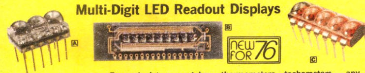
Radio Shack’s 1976 catalog featured magnified LED displays.

Early LED displays often had all the diodes on a single die to reduce cost. That made them very tiny. It wasn’t unusual to see displays with magnifying bubbles to make it easier to read.

The important point isn’t whether they used exactly seven segments. Many didn’t. Some divided the numerals differently or used additional pieces to produce more attractive typography. The insight was the same: begin with the most complex digit and selectively remove strokes to create all the others.

Why Seven?

One of the reasons seven segments became the standard is that they strike a perfect balance (although not everyone agrees, as you can see in the video below). With fewer than seven elements, several decimal digits become difficult to distinguish. Adding more segments certainly improves appearance, but every additional segment increases wiring, decoding logic, manufacturing cost, and the number of possible failure points. Seven is the right number for — um — numbers. But what about letters?

You can make some compromises to show some letters. For example, old computers would display hex digits using seven segments, but the A would be uppercase and the B would be lowercase. You also had to light the top segment for the 6 to make it look different from a B. But you only need A-F for hex. If you need, say, the letter S, there’s no real way to make it not look like a 5 with 7 segments. But sometimes, the letters you can make are good enough.

There were also 8- and 9-segment displays that could do better with letters and special characters. You can increase the segments further to get more glyphs.

The Union Jack

Different segment counts for displays (public domain by [errorage])
The solution for full letter displays was to add more segments. Despite Mason, you didn’t really need 21. By the 1970s, fourteen-segment and sixteen-segment displays had become common in instruments, telephones, calculators, and video cassette recorders. Their pattern of diagonals and crossbars earned them the nickname “Union Jack” display because the arrangement resembles the British flag. These are also sometimes called starburst displays. You occasionally see 16-segment displays, too.

Even Today

Today, you have a plethora of options for adding alphanumeric screens to just about anything. Yet, you still see 7-segment displays hanging around.

The seven-segment display isn’t successful because it’s beautiful. It isn’t even especially flexible. It’s successful because it’s close to the minimum solution that works. It delivers readable numbers with very little hardware, whether the technology behind it is incandescent bulbs, neon, vacuum fluorescence, LEDs, LCDs, or even ink on a printed price tag.

Perhaps that’s why it has survived every technological transition for more than a hundred years. Good engineering ideas often outlive the technologies that first bring them to life.

And once you start looking for segmented displays, you’ll notice they’ve been hiding in plain sight for much longer than the digital age.

Featured image: [Arduino Enigma]’s marvelous Seven Segment Art Installation

Is Now the Time for Volumetric 3D Printing?

By: Ian Bos
7 July 2026 at 10:00
Art of 3D printer in the middle of printing a Hackaday Jolly Wrencher logo

Of all innovations adopted by the maker community within the past couple of decades, one stands among the rest on top for anything regarding manufacturing. It goes without saying here at Hackaday how many projects have been reliant on using the technology to turn their ideas into reality. 3D printing has been a maker community invention and, in return, has expanded this hacky community into something that anyone with an imagination can get into. It also goes without saying that the layer-based tech imposes limits on what we can actually create: think overhangs and layer adhesion. However, there’s a possibility that a recent offshoot of this scrappy community has the power to eliminate some of these faults.

Volumetric additive manufacturing (VAM) is a young technology that has a similar start to many new tech toys, including the original SLA of the first 3D printers. That is expensive and completely stuck in the laboratory… Fortunately, that’s not where 3D printing as a whole stayed, as the RepRap project managed to bring the obscure technology to the hobbyists’ main stage. An entire group of people formed and spent countless hours until the useless pieces of poorly extruded plastic could form parts impossible to make with anything else. A cool quirk of history is that it likes to repeat: examples spur recreation, and this appears to be happening with the technology found within VAM printing.

History

Hold up for a second. While we have covered VAM here before at Hackaday, it’s not exactly the most well-known tech or the easiest to understand. So what is it? Starting from the beginning and simplest forms, VAM is similar to the more  common SLA printing. Using a light source and light sensitive resin, both of these methods can create entire physical objects by solidifying or curing specific areas of a vat or vial of resin. SLA will often use something like a laser and layer by layer “draw” the model until the entire geometry is finished. A quirk of most of many photosensitive resins is that they need to overcome a threshold before they can start curing. This allows VAM to do something a bit different. The earliest methods of VAM used intercepting lasers which allowed selective curing only where these beams were intercepted. One singular spot at a time would be able to overcome the threshold required for printing, allowing you to build up most geometries.

Xolography Print

This works, but for more complicated models there’s more effective methods. One type has been covered here before called Xolography, still using intercepting beams, however with differing wavelengths which allows for more finite control. This is effective, but the resin is complex, requiring two-wavelength-photon-sensitive photoinitiators. Introduce the current standard in VAM printing, computed axial lithography (CAL). This method finds itself using existing methods found in traditional tomography, such as CT scanners. CAL methods are basically reverse tomography, where a model is used to create projections to be projected in printing. These projections allow dose control in each “voxel” of resin from changing the projection as the volume of resin is rotated. When ideal, this means that the entire model is printed at once. No layers needed for printing, and printing in minutes rather than hours.

Open-Sourced

Cool, but why should you care about this tech? Because you could start using it now! Just like the RepRap project before it, VAM has OpenCAL. OpenCAL was started by the same lab that originally created the axial version of the technology. UC Berkeley released the first OpenCAL around 2019 which was… well a start.

Functionally practical for only big budget research, it was far too expensive and complicated for any hobbyist with a 9-5 to realistically touch. Last year saw a new model presented at Open Sauce which used a consumer projector and common hobbyist electronics. While this was an improvement, there are three barriers to VAM printing; the hardware, software, and chemical resins make it a challenge for any individual alone. A newer version of the hardware was quickly put together for this summer. This helps with the hardware element, but there’s two new aspects being released alongside OpenCAL V2 for other unsolved problems.


Software: Tomo

Tomo with the Thinker model being prepped

For a little while now there have been various software packages available for allowing easier use of whatever VAM printer you might have, however these had various problems. From being undocumented to being complicated for anyone without comfort in command line , something different would be needed. A standalone application would certainly work, and low and behold that’s exactly what’s being tried here, called Tomo. Tomo allows you to use an OpenCAL printer with little thought or expertise, or ideally any other type of VAM printer.

Chemistry: Formlabs Resin

Large form factor VAM print

Material science is always a particular challenge for the open source community. Unlike software, you can’t distribute unlimited copies of your perfect mix of photosensitive resin without special chemical clearances and certainly not for free. Some of the first 3D printers from RepRap would use a nylon weed wacker line in place of the standard PLA of today. Unfortunately there’s less flexibility in the fine tuned resin found in VAM. This resin has to have a nonlinear photo-reaction for selective curing, be fairly transparent to the reactive wavelength, and be very viscous to prevent resin movement during printing. Formlabs, which makes resin printers and resins, has gotten into the act. Through talks between the OpenCAL team and Formlabs, an agreement for production of this special resin is being worked out, allowing for far cheaper material.

Hardware: OpenCAL

OpenCAL V2 printer
OpenCAL V2 printer

Of course this leaves the printer itself. OpenCAL is designed for a variety of different sized printing volumes, projectors, or anything else you might have in mind. Expect printing anything from this printer to finish in the span of minutes. While it can do the same small prints found in the older model of OpenCAL, experiments involving larger form factors have been attempted. But if you want more details make sure to check out the documentation here or join their Discord channel!

Future of VAM Printing

So how far can this technology really go? Could it pass traditional methods of 3D printing? Well, it’s certainly faster than traditional printing, however, there’s still plenty of trouble when trying it out. How do you remove partially cured resin off your print? How do you actually tell when the print is done? These are problems that are being fixed right now by the community, and maybe you can be the one to fix something holding it back. It’s fair to say that the community that has propped this technology up to where it currently stands is who is going to decide where it goes.

Ultra-Long Range Flights To Ease Australian Air Travel

6 July 2026 at 13:00

Pity the poor Australians. Isolated on a jagged hunk of land far from everywhere else, these industrious people have to take two-legged flights (or more) to reach a great many destinations in the northern hemisphere. It’s expensive, time consuming, and makes planning a trip a complete headache when wars break out around popular hub airports.

One airline is trying to solve this problem. The nation’s flag carrier, Qantas, has been hard at work on Project Sunrise. The goal is to run some of the longest non-stop commercial passenger flights ever, with great effort going into solving the technical and economic challenges involved.

No Stops

When travelling from Australia’s major capital cities, flights to destinations like London, the rest of Europe, or the US, all involve stopovers in intermediate airports along the way. A great many routes stop in Dubai or Qatar, while others transit through Hong Kong, Singapore, or Thailand. The need for stopovers complicates air travel for the passenger, particularly when delays cause missed connections or baggage gets lost from one flight to another. It can also just be tedious—sometimes a stopover can last 10 hours or more, which is an incredibly uncomfortable amount of time to spend in even the nicest airport. The reason behind stopovers is simple enough—the average commercial airliner just doesn’t have the fuel range to haul many hundreds of passengers from Australia to Europe in a single hop.

Qantas has formerly run long-range routes with Boeing 787-9 aircraft, but they lack the legs to make it from east-coast capitals to major international destinations. Credit: Qantas media resources

Qantas has been trying to improve Australia’s passenger airline links for quite some time by finding ways to eliminate these tedious stopovers entirely. Thus was born Project Sunrise, which hoped to find more direct routes between popular world cities and suitable airliners that could fly those routes without stopping.

An early 2019 test flight probed the practicality of flying from New York to Sydney in a single hop. Due to the limitations of contemporary aircraft, sacrifices were made to get the flight over the line. Where the Boeing 787-9 would normally carry up to 280 passengers, the test flight would only haul 40 to save weight, and thus save fuel. No cargo was on board, and the tanks were brimmed to ensure maximum range was available. Even then, the 16,250 km route was considered to be at 115% of the plane’s normal range, and there was only 90 minutes of contingency  when it came to fuel onboard if something went awry. Despite the challenges, the test was a success, and provided useful learnings on how to handle things like crew fatigue on a 19-hour continuous flight.

Qantas was also experimenting with practical revenue services at this time, too. In 2018, the airline had established a direct route from Perth to London, flying the Boeing 787-9 in a 236-seat configuration. Flying the 14,484-kilometer route was just within the practical range of the aircraft. It was a useful route that made travel easier for passengers departing Australia’s west coast, but far from the golden ideal of allowing direct flights to major international destinations from the major capitals of Melbourne and Sydney. The route has also since fell victim to geopolitical strife, as the Iran War shut down large swathes of airspace in early 2026. Qantas was forced to alter its flight paths, which added 30 to 45 minutes to the usual flight time—just enough to tip the route over the practical limitations of the aircraft’s range.

Future Goals

However, the crowing achievement of Project Sunrise is still yet to come. 39% of Australia’s population is concentrated in Sydney and Melbourne alone, with both capitals situated on the country’s east coast. It would be most advantageous from a business perspective for these cities to have direct links to major world destinations, and it would benefit the broadest swathe of Qantas’s customer base. Only, the problem comes back to geography, with these two capitals being over 16,000 kilometers from popular destinations like New York and London.

Aviation Photographer London - Stuart Bailey Photography
The A350-1000ULR is key to Qantas’s efforts to launch non-stop services to far-flung destinations. Picture Credit: Stuart Bailey, via Qantas media resources

Qantas has risen to the challenge, regardless. The airline challenged both Boeing and Airbus to develop aircraft intended to fly routes from Sydney, Melbourne, and Brisbane, to destinations like New York, London, Cape Town, Paris, and Rio de Janeiro. This was later whittled down to a narrower focus on the Sydney to New York and Sydney to London routes. Airbus would come out victorious, with Qantas ordering twelve examples of the Airbus A350-1000ULR. The specially-configured model features an additional rear centre fuel tank and a higher maximum take-off weight in order to fly routes up to 22 hours non-stop, along with a reduced seat configuration serving just 238 passengers. The extra range makes for a huge difference compared to more conventional routes out of Australia, which often pair two flights up to 14 hours each. The extra range of the new aircraft saves passengers both hours of flight time, along with the hours normally spent sitting around on layover in a hub airport along the way.

The new aircraft has been undertaking test flights ahead of a planned 2027 launch of revenue services. Credit: Qantas media resources

A typical flight from Sydney to New York or Sydney to London is expected to take 19 to 22 hours. The no-stop nature of the route will enable 99% of Australians to access either destination either direct, or with one-stop—such as by flying in from another major capital on a domestic flight. The flights are expected to run with a higher-than-usual ratio of premium seats, based on the expected demand for these services.

The main thing holding back the new service is aircraft delivery. Production is underway in earnest, with the first A350-1000ULR to be delivered in April 2027. Daily non-stop flights between Sydney and London will begin from October 2027, with tickets to be on sale from February.

Aircraft cabins will be optimized to have more space and amenity to keep passengers comfortable on ultra-long-range routes.

The new Project Sunrise services will be a gamechanger for many people travelling to and from Sydney, and other Australian capitals. It will relieve a major pain point—layovers—that have become a dreaded fact of life for Australians headed far abroad. It will still perhaps be some time before Australians get more direct services to a wider range of destinations, because these new services will have to prove themselves. If the passenger numbers aren’t there, the services won’t make money, and it may not prove worth the hassle to operate these ultra-long-range routes. If, however, convenience truly is king, then there may be much greater investment in this area to link Sydney and Melbourne with more cities directly. The only losers in this case will be the hub airports across the world, which will grow just a little quieter for the loss of Aussie accents in the terminal.

Know Your Food: Organic Production

2 July 2026 at 10:00

A few weeks ago we published the first in a new series of articles, Know Your Food. It was born out of the realisation that most people know surprisingly little about what they eat, and to apply a bit of Hackaday curiosity to received opinion on the subject. As we put it then: “To know both how common foodstuffs should be made, as well as how they are made industrially, should be an essential for everyone” We’ll continue in that vein, with a look at organic food.

If you buy your food in a supermarket it’s likely that in the vegetable aisle you’ll be presented with a choice. On one hand you will have the normal vegetable, and on the other and usually for a slightly higher price, the organic version of the same vegetable. What’s going on?

So What Is This Organic Stuff All About?

A watercolour picture of a bucolic scene with a farmhouse surrounded by trees, and some cows in the foreground.
It is unlikely that a typical organic farm in the 2020s will resemble this John Constable painting. John Constable, Public domain.

Organic production is a system of agriculture that emphasises natural fertilisers, pesticides, and farming methods over synthetic or intensive ones. It has its roots in the first half of the 20th century, and as the decades progressed it has become an important sector of agricultural industry. I grew up steeped in organic agriculture because my grandfather was an early adherent in the years following the war, so I’ve seen it from the sharpest end. There is a lot to commend organic production for and plenty of reasons to embrace it, but with that come some problematic aspects, and even dubious claims. Here I’ll try to unpick some of that.

It’s tempting to believe that all organic production is somehow a return to a 19th century rural idyl, complete with the obligatory chickens in the farmyard. Some organic producers do take a slice of this back-to-the-land approach to their craft, but the reality of organic farming is a very modern approach to managing the ecosystem. Organic farmers are not wary of progress, and neither are they reluctant to use pesticides or other chemicals. Instead they do so according to the principles of organic agriculture, so any techniques they use are designed to be beneficial to the ecosystem, and any chemicals have a natural origin.

The rear view of a tractor towing a manure spreader driving away from the viewer while spreading manure onto a grass field. It's a misty winter day, and leafless trees are visible in the distance.
If you spend time around organic agriculture, you become a manure expert. Ray Bird, CC BY-SA 2.0.

An important thing to understand is that the line between organic and non-organic agriculture is not sharply drawn. Crop rotation for example is long established farming practice, as are techniques such as contour ploughing in areas with soil erosion. As for fertiliser, there will be very few farming operations whose work does not include manure in some form, or who do not take advantage of nitrogen fixing crops. Pesticides such as the insecticide pyrethrum – originally derived from chrysanthemum root – or Bordeaux Mixture as a fungicide – a solution containing copper ions, so called because of its origin in French vineyards who applied lime solutions from copper containers – find uses where applicable in both organic and conventional agriculture. The important distinction lies in the organic farmers not going further than this, into synthetic amonium nitrate fertiliser for example, or glyphosate herbicide, which you might know as Roundup.

That’s the organic sales pitch, and it’s a compelling one. Now, we’ll go through the not so positive aspects, both of the movement and of the business.

Organic status is not simply conferred to produce by virtue of being organically grown. Instead it’s a legally protected designation, enforced through a system of certification performed by designated organisations. Where I grew up in the UK for example, organic certification is performed by the Soil Association. This is good because it preserves trust in organic status, but it suffers the flaw that it’s a profitable business for the certifier, and an expensive one for the producer. This in turn favours larger producers who can afford certification, and leaves the smaller producer unable to afford certification and thus unable to label their produce as organic. They can describe it as “Organically grown” of course, but they lose the cachet of the organic label. Since many small producers are by necessity organic, this affects a large number of producers if not a significant sector of the market.

Is Organic Food Really Better?

Then there is the produce itself. Is it better than the non-organic stuff? Here we enter complex territory, because the answer differs depending upon the circumstances.

In terms of what advertising people like to call “goodness”, by which I mean nutrients, vitamins and minerals, and the like, in many cases it’s difficult to make a case for the organic product being superior to the non organic one. There will be exceptions such as apples, where a typical non-organic commercial dessert apple is overwatered to the point of diluting the beneficial properties it might have in search of the elusive “crunch”. But in the more ordinary case, that organic zucchini is unlikely to have more nutritional value than its non organic equivalent. It’s important to note that the organic product will lack any pesticide residues which may be present on its non organic equivalent, however it must be remembered that pesticide residue levels in food are subject to their own stringent regulation.

A sign advertising Wynford Farm Shop, selling local Organic Aberdeen Angus beef.
If you’re looking for the best organic food, seek out places with signs like this. Stanley Howe, CC BY-SA 2.0.

In terms of flavour, yet again it’s a mixed bag. An organic product grown in as intensive a manner as can be got away with under the rules, is not likely to taste better than the equivalent. It’s difficult even to pin down what in the husbandry governs the flavour of the finished product in a scientific sense, however as someone who grew up around organic production I’d offer the view that the longer something took to produce, the better its flavour is likely to be.

The Slow Food movement champions products made in this way, usually traditionally produced foods, heritage varieties, and foods with a particular terroir. If you’re looking for better tasting food then you may not find it with a supermarket organic label, but it’s quite likely that one of those small organic producers will have what you are looking for, simply because their methods are less intensive.

Finally, if you’re looking at the benefit to the environment, it’s likely that in most cases the organic product will impose less stress on the ecosystem and the wider environment than its non organic equivalent. If that’s your concern you should also look further than the means of production and into food miles; how far did the food in front of you travel to your plate? Here in Europe the strawberry is in season from around May to September, so does it make sense to fly them from the other side of the world in January, however nice they taste?

So now I hope you have more of an idea about organic food than you did at the start of this piece. You’ll know something about its benefits and problems, and you’ll know when it’s better than its non-organic equivalent. I hope you’ll find the food you like, and if you do, I hope it’s from a small producer, they need your business. Bon appetit!

Header: MichelM10, CC0.

UDP Broadcasting and Easily Finding Network Services

1 July 2026 at 10:00

Local area networks (LANs) that use technologies like Ethernet and Wi-Fi are incredibly useful for letting devices talk with each other. Yet a core problem here is knowing which devices are where on the network, as anyone who has ever tried to add a network printer or network share to their system can probably attest to. Unless you happen to know the IP address of the LAN device, the port, and protocol, the target device may as well be located on the Moon without further help, such as automatic network discovery in lieu of waddling over to the device and reading the label listing its IP address.

Over the decades quite a few ways have been developed to enable such network discovery, with many of them using UDP broadcast as the first step. By broadcasting a global message on the entire LAN, any device that has an actively listening UDP socket on that particular port can parse said message and decide whether it’s feeling sociable enough to reply.

The topic of UDP broadcasting is however not as straightforward as it may sound if you’re just getting started, including the existence of many opinions on the ‘right way’. There is also a massive divide between a sprawling service discovery protocol like mDNS and a light-weight one like that one that I had to implement a few years ago for an open source project.

Network Broadcasting

The obvious advantage of a broadcast message is that a client device that seeks its protocol soul mate on the LAN doesn’t need to ping all possible IP address and subnets. Instead,  a broadcast message is designed so that all connected networking devices know that it should be forwarded to all other known devices. Thus with a single message from the client, in theory, only a single message will then neatly land at every single other connected system.

Of course, this ignores happy joy fun things such as convoluted network configurations, such as those involving overlapping Wi-Fi repeaters and subsequent routing, but in general we can assume that this is how it works. Various edge cases and fascinating complications of these will be considered in a later section.

Much of this service auto-discovery is tossed under the header of ‘zero-configuration networking‘, or zeroconf for people who don’t like typing. The best part about zeroconf is probably that there are so many standards here, ranging from DNS-SD to mDNS, UPnP, SLP and others. Perhaps unsurprisingly, one of the major issues here is that platform support here is spotty, with mDNS – despite being one of the most universal – not having much support outside of MacOS/OS X with Bonjour and Linux/BSD with Avahi.

Thus while trying to add the auto-discovery of NymphCast receivers and media servers by NymphCast clients, I found myself asking the daunting question of whether I was at risk of being about to embark on reinventing the proverbial wheel. After all, nobody wants to become the subject of an xkcd comic.

UDP Discovery Basics

As it turns out, I ought not to have been too worried, as despite looking everywhere I could find nothing along the lines of the NyanSD network service discovery (NSD) protocol that I ended up implementing and integrating into NymphCast. What I wanted after all was the most no-frills NSD possible that could be easily integrated, while working the same across just about any desktop, server and embedded platform imaginable.

All that’s needed for this is a way to create an appropriate UDP socket, and a way to either broadcast a query and receive the response, or to listen for incoming UDP packets. Here you can figure out the platform-native method for each target platform, or not reinvent the wheel and use an existing networking library for C++ like Poco. This is what I used for NyanSD, along with my ByteBauble utility to handle endianness conversions.

For the UDP server — the listening side — the procedure is fairly standard, with a regular UDP listening socket. As UDP is a connectionless protocol, there is not a lot of preamble here, just a UDP socket instance (here Poco::Net::DatagramSocket), which is bound to the target port and regularly polls for any fresh UDP packets to process. This can all be seen in the single source file for NyanSD which covers both the client and server side code.

Where things get spicy is with the client that sends the broadcast query and waits for any replies. If we were to just shove the query data into the socket along with the request to toss it over to a regular IP address, not a lot would happen. To make it into a broadcast request we need a few things:

  1. Let the network subsystem know that we want to do broadcast things.
  2. Create the special broadcast address for the target network interface.

With Poco the first point is easily handled by simply calling setBroadcast(true) on the UDP socket instance. For BSD sockets this sets the appropriate flag on the socket, which is essentially repeated across all OS implementations due to how prevalent the BSD socket library is.

The second point can be summarized for IPv4 as a curt ‘make it end with .255’. For example 192.168.0.255 when the client network interface’s IP address is 192.168.0.42. If there are multiple interfaces on the client system, you can go through the list one by one to broadcast on each of them before filtering out potential duplicate returns.

As for how to do broadcasting with IPv6: you don’t, as this protocol relies on multicast and special multicast receiver groups, which is another kettle of fish and of not much relevance for LANs.

Complications

If you look at the NyanSD API, it may give the impression that the query process is incredibly straightforward, with the sendQuery() function neatly returning a stack of remote systems that responded to our query. While these are definitely all the responses, it’s important to remember that NyanSD queries every single network interface. This means that the responses are likely to contain duplicates, which may even come from the loopback address when a service runs locally.

The filtering of this is captured in the NymphCast client library (libnymphcast) where the findServers() function in the main source file calls the isDuplicate() and isDuplicateName() functions, as well as the removeLoopback() function that nukes any responses that match a remote service found via a non-loopback interface. This last filtering is essential for NymphCast when e.g. using playback groups that would otherwise get confused by a stray loopback address.

Although one may think that such in-depth filtering is unnecessary if all you have is a single Wi-Fi or Ethernet interface in your system, one of the curveballs that I encountered during real-life testing was apparently related to Wi-Fi repeaters. For some reason it seems that the way that the repeaters did their broadcasting led to erroneous duplication of packets and thus multiple returns from a single system.

Depending on your exact use case and network configuration you may encounter any such issues and perhaps an exciting new one.

NyanSD Findings

Over the years that NyanSD has been used in the NymphCast project, it has proven to be one of the most reliable and probably nearly zero-fuss components. I have so far used it on Windows, various Linux distributions, FreeBSD, Haiku, Android, and the ESP32 via FreeRTOS and ESP-IDF. What this experience has proven to me most of all is that service discovery doesn’t have to be complicated.

The basic UDP protocol is simple and reliable enough that, barring a very sick LAN, there shouldn’t be any issues here. Assuming you get your filtering sorted of the responses, it’s probably the last part of a project to worry about.

One thing that I’m also very happy with in NyanSD is that there’s no set port in the protocol, like how mDNS always uses port 5353. What this means is that I can have NyanSD listen with a UDP socket on the same port as the NymphCast server’s TCP socket, which also means that different services with their own port can be targeted directly rather than every NyanSD-enabled service on the network getting blasted by every NyanSD query.

I did also do some work on a NyanSD daemon as a more central services database, but so far I have had no real need for it in a practical deployment. I guess that such a thing could be very useful if the port of a service is not set in stone, but generally that’s the one aspect of network services that tends to be boringly predictable.

How Airspeed Sensors Work

30 June 2026 at 10:00

When you’re driving your car, you’re probably regularly looking at the speedometer to make sure you comply with the local speed limits. The method by which it works is simple enough: the rotation of the wheels is sent mechanically via a cable to a dial on the dash, or an electronic sensor counts the rotations of the drivetrain and an electronically-controlled needle or display shows the speed.

But what about if you were in an aircraft, and the wheels had nothing to do with how fast you were going? How would you even begin to measure speed? There are two ways: there’s a convenient solution to this problem rooted in simple fluid mechanics, and a far-more-complex modern solution. Today, we’ll explore how planes and helicopters are able to figure out how fast they’re going, by the old ways and the new.

Classical Methods

Measuring airspeed can be achieved by measuring stagnation pressure with a pitot tube, and comparing this to static pressure. This can be done at different points on the aircraft, or a pitot-static tube can be used, which measures both stagnation pressure and static pressure in a single probe. Credit: Chaos386, CC BY-SA 3.0

A key thing most aviators want to know is how fast their aircraft is going. Specifically, it’s nice to know how fast it’s moving relative to the airstream around it, which is referred to as airspeed. This is important, because it’s the aircraft’s velocity relative to the flow, such as wind, that determines the performance of the airfoils, how much lift is generated, and whether or not the aircraft is approaching a stall condition where it might fall out of the sky.

Bernoulli’s equation, rearranged to find airspeed (u), by subtracting static pressure from stagnation pressure, multiplying it by 2, dividing by fluid density, and taking the square root of that result.

Measuring airspeed is most commonly achieved with the use of a device called a Pitot tube. The pitot tube is a tube with a hole in one end that points directly into the airflow in the direction of travel of the aircraft.

As air flows in, it reaches a dead end and the flow slows to a stop, or stagnates, since it has nowhere to go. This allows a pressure sensor or a manometer or other device to measure the stagnation pressure at this point. The stagnation pressure measurement is related to the flowspeed of the incoming air since the kinetic energy of the flow is converted to pressure as the flow comes to a halt.

A secondary tube, pointing perpendicular to the airflow, is then used to measure the static pressure of the surrounding air, without the ram effect of the air being forced in by the aircraft’s forward motion. Then, it’s possible to calculate the velocity of the aircraft relative to the airstream by plugging the stagnation pressure and static pressure into a rearranged Bernoulli’s equation.  If the pitot tube and static tube are hooked up to electronic sensors, the airspeed can be calculated electronically, and fed to a display or digital gauge.

A classic airspeed indicator has the pitot tube and static tube feeding right into the gauge in the cockpit. The pressure differential causes the diaphragm to expand as the airspeed increases, which mvoes a mechanism causing the needle to move on the gauge. Credit: FAA, public domain

Alternatively, it’s possible to effectively do this “calculation” mechanically. In earlier days, static and stagnation pressure captured by each tube would be fed to a gauge. Inside, the stagnation pressure would be fed to a diaphragm which moved due to the difference relative to the static pressure which is fed into the gauge body, and the movement of the diaphragm would, via a simple mechanism, shift the needle on the gauge.

A small General Aviation aircraft might mount a single pitot tube on the aircraft, feeding the air speed instrument in the cockpit. Commercial aircraft might mount two or more for safety’s sake, in case one becomes inoperable, while large airliners may have four or even more to provide a high level of redundancy and error checking. Heaters are commonly included on pitot tubes to ensure they can be kept free of ice, which can otherwise completely block a tube and make it impossible to obtain an airspeed reading.

Pitot tubes sticking out in the airstream underneath a Boeing 777-381. Credit: Cassiopeia sweet, public domain

For pilots, not knowing how fast (or slow) the aircraft is going can be highly dangerous, as it can lead to entering unstable flight regimes such as stall. Thus, it’s imperative that the pitot tubes remain unobstructed and functional for safe flight. Many aircraft accidents have occurred because of blocked or malfunctioning pitot tubes or airspeed instruments.

The New Way

Of course, you could fuss about with pitot tubes and pressure sensors and deicing measures, but that’s all very fiddly and old hat. There is an entirely different way to figure out a plane’s speed, though it’s only been available for the last few decades. It’s as simple as throwing a GNSS receiver on the aircraft.

Yes, whether your particular poison is GPS, Baidou, GLONASS, or Galileo, any major satellite navigation system will be able to tell you the speed of your receiver. Simply measuring the change in the receiver’s position over time is enough to calculate out the speed, and any off-the-shelf receiver will present this information as standard. It’s generally not used as a primary indicator in aircraft, because it reports ground speed, not airspeed, the latter being more relevant for aviation purposes. Still, it can prove to be a useful sense check when traditional airspeed indicators are non-operative or reporting confusing data, and GNSS devices are widely used on many aircraft today.

Flying High

Many modern aircraft have so-called “glass cockpit” displays that include feeds from GNSS receivers, which can provide supplementary data such as satellite-based ground speed measurements. However, these readings are generally not used for the primary task of flying the aircraft. Credit: Bluedisk, CC BY-SA 3.0

If you’ve ever wondered how an aircraft measures its speed as it floats through the amorphous gas cloud we call an atmosphere, now you know. Even to this day, where electronics and computer wizardry control our fanciest aircraft, airspeed measurements are still done with the same simple physics, just with some fancier sensors for help. The fundamentals haven’t changed at all. Now you know, you can always dig deeper into the many other rich applications of Bernoulli’s equation and fluid mechanics in general. Happy learning.

❌
❌