After the Orion capsule of the Artemis I lunar mission returned to Earth, it was found that massive chunks of its heatshield had been ripped off, posing a serious risk to any future missions. In a recent video in which [polymatt] takes a break from repairing old laptop shells and the like, he tries to recreate the Orion’s heatshield using a variety of methods and materials.

For this test a number of samples were created, each using the same kind of segmented structure as the larger Orion heatshield. The filler was created from the published materials for the heat shield by NASA, requiring just serious mixing.

The resulting samples were then cured with thermocouples inserted, before they got blasted with the heat from a propane torch, trying to simulate the various re-entry patterns.

Perhaps unsurprisingly, the results matched the findings by NASA for why the Orion’s heat shield had failed, being the build-up of gases due to the sustained pyrolysis processes that eventually fractured the material. Despite some experimental flaws that injected residual heat from the copper structure, this still seems to be a pretty good setup to test ablative heat shields in DIY lab conditions.

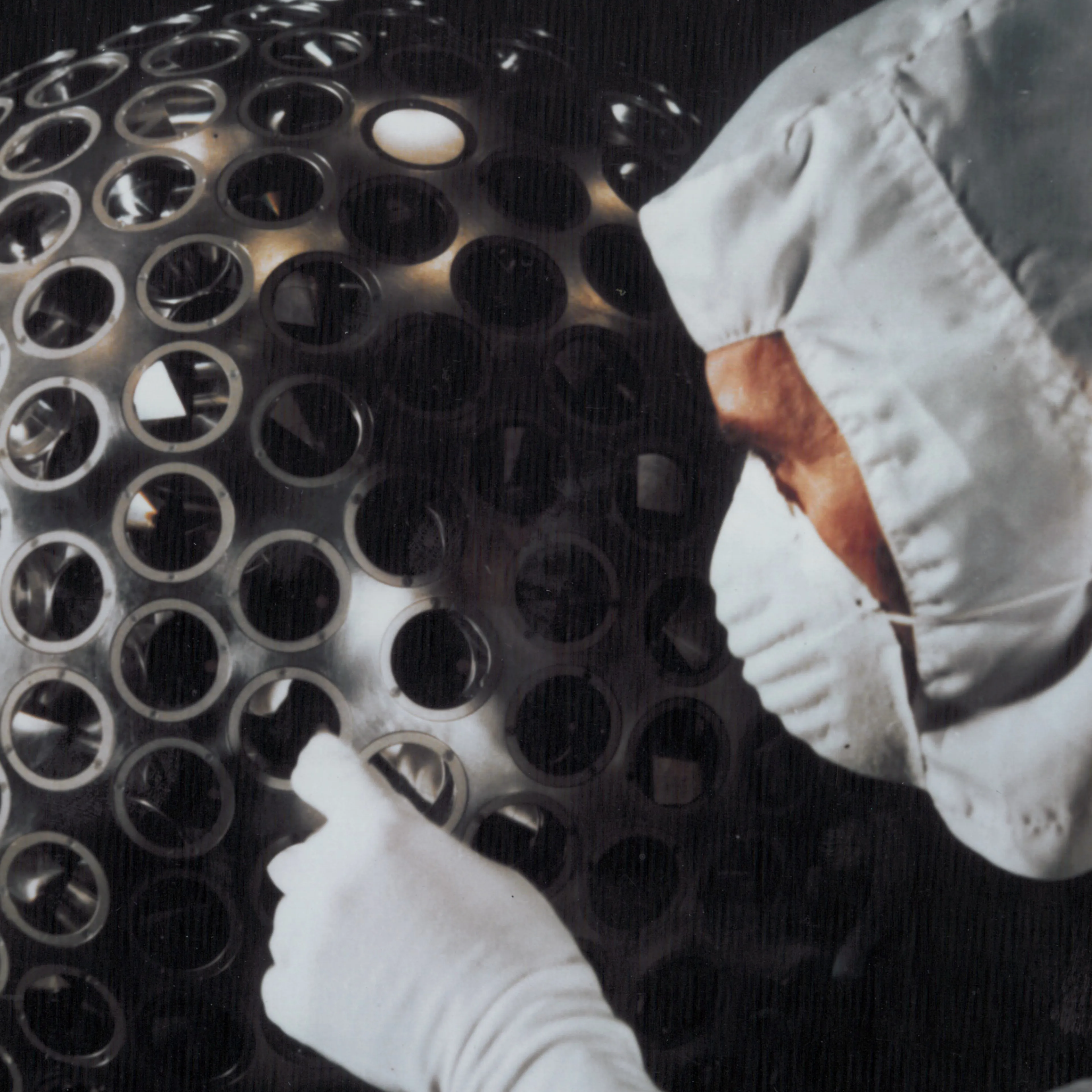
Launched in 1976, LAGEOS-1 (LAser GEOdynamic Satellite) is unusual in that it contains no instrumentation, no electronics, no power supply, and no means of propulsion. It’s spherical, weighs just under 407 kg, and looks a bit like a disco ball. It may not be accurate to say it does nothing, but unlike most satellites its role is entirely passive. It’s also one of the oldest scientific satellites still in service.

The lens-like objects covering the surface of LAGEOS-1 are corner cube retroreflectors, which have the nifty effect of always reflecting incident light right back towards its source.

Ground stations fire short laser pulses at it and measure the time it takes for the light to return, a form of time-of-flight ranging. Since LAGEOS-1’s orbit is highly stable, it provides a reliable reference point for measuring even tiny changes in the Earth itself. The size, shape, rotation, and more of our planet can be measured as a result. LAGEOS data (LAGEOS-2 was launched in 1992) has also been used in tests of general relativity.

Its orbit and construction were deliberately chosen so that atmospheric drag and other disturbances would be minimal. The simple, maintenance-free design combined with an extraordinarily stable orbit means LAGEOS is expected to circle our world for millions of years to come.

LAGEOS-1 also contains a message to the future in the form of two identical plaques prepared by Dr. Carl Sagan just in case there’s anyone around to find it some day. Check out the short 1975 video from NASA, embedded just below.

A few weeks ago, my wife was out walking the dog, and she sent me four or five photos of small orange boxes planted all around our neighborhood. (OK, I’ll bite!) They had little cards on them explaining that they were geophones, and a QR code on them that lead to a website with all the details. Munich was getting a large-scale seismic survey to map out our underground water, with the aim of using it for geothermal heat and power in the near future.

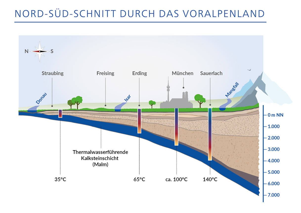
How do you map up to five kilometers under the earth? You pound the ground, sending shockwaves downward, and then listen for their reflections. At the boundaries between different layers, the change in the speed of sound in the different media cause reflections. Calculating the time it took for a given reflection to reach you lets you figure out how deep the layer boundary is.

The seismic survey procedure goes like this: geophones are set out at roughly 20 m intervals in lines spaced around 300 m apart that run roughly north-south, while “vibrotrucks” drive a roughly east-west course, creating mini-earthquakes every 20 meters along the way. Covering a surface of 1,000 km^2 with over 120,000 sample locations and exciting them 86,000 times is going to take a while. Lucky for me, they started in my part of town.

Hot Water

Because the earth is essentially a ball of hot molten metal with a thin and crispy outer crust, and because there is radioactive decay going on even within the crusty bit, temperatures rise as you dig down: roughly 30 °C per kilometer. And Munich has this fantastic source of water that’s folded under the earth in a layer that dates back to the Jurassic, which makes it both low in dissolved minerals and sitting just around 3 km down: at 100 °C. This turns out to be the sweet spot in terms of difficulty of drilling and heat gained from doing so.

Blessed with hot water underground, the question is how to best use it. The plan at the moment is to situate a number of geothermal plants around the city, drill relatively large bore holes at each site that reach down 1 km to 2 km, and then drill diagonally down after that to spider out into a larger source of water. This “extended reach drilling” pulls from a larger heat source, prevents cool spots, and has only recently become technologically feasible.

Which brings us to the GIGA-M study. A 3D map of the underground will help plan out where to put the geothermal plants, in which directions the runners will need to be drilled, and generally how to best coordinate the resource. There were a number of individual smaller surveys done over the last 20 years, and Munich and the surroundings already have a number of geothermal plants, but this survey aims to fill in all of the gaps.

The Hunter and His Prey

It was a Thursday morning when my wife thought she heard some pounding and humming outside. She was wrong, but it got us to look at the online map, and while they weren’t in our neighborhood just yet, they were probably within easy driving distance. I threw my camera and tripod in the car and headed out.

Out in the country, just outside of Grossdingharting (you can’t make these names up!) I spotted a plume of dust rising up from a field. Was it just a farmer tilling? Or was it a vibrotruck? I drove through the woods on a logging road, and when I came out, I was nearly face-to-face with the beasts.

They were loud, and I felt the rumble when I stepped out of the car, so I ran up and asked if I could film it. They said “sure”, and I set up the tripod. The first video I shot, apparently I hadn’t screwed the camera down hard enough in the tripod, and it vibrated loose. So I ran another 20 m further and tightened everything down.

I’m not going to lie: it was exceedingly loud and very exciting. I drove back home and couldn’t wait to review the footage.

The next morning, I heard the same sound outside my own house. They were driving vibrotrucks around in the field about a block up the street. I grabbed the camera and ran out barefoot to get footage. And then Saturday morning, while cooking blueberry pancakes for the family, they drove up my street. Am I stalking the vibrotrucks, or are they stalking me?

An engineer asked if they could stand in our front yard, so I took my chance to bombard him with questions. He seemed stoked to talk about it.

Geophones and Vibrotrucks

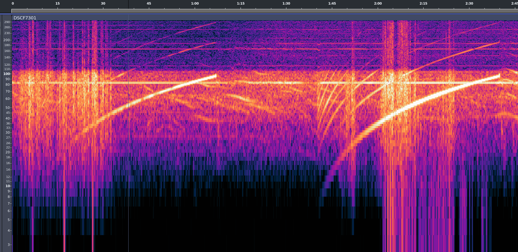
When you stand next to one of these things, first it shakes, and then you can hear a bassy tone, and then it rises and stops. They’re obviously doing a frequency sweep, much like you would use a sonar chirp to help disentangle the multiple reflections from one another.

The sweep means that even if they receive two reflections at once, they will hear two different pitches because one signal traveled further than the other, and comes from the earlier, lower-pitch part of the impulse. It also makes for a very easy to find signature. Correlating these times of flight across the entire array of geophones gives a 3D map of the underground layer discontinuities.

You can see from a cleaned up version of the audio that they’re sweeping from something like 6 Hz up to maybe 96 Hz.  The lower end sounds like distinct hammering, and the top end a humming. Here is another video, with filtered audio. Because you feel the vibrations through your feet and in your chest, the live experience is a little bit like this with more noise. Play on good headphones or with a subwoofer for maximum effect.

Of course, the time of flight matters. I asked if each geohpone had a GPS timebase, and the friendly engineer told me that they individual geophones don’t – too expensive – but that when they install one, they connect it to a laptop with GPS that records the location and sets the geophone’s clock. When they harvest them, they record the location again, dump the time to verify that the clocks haven’t drifted too much, and then pull down all of the recorded timestamped data.

Why do they drive around in pairs? It’s simply because they make twice the vibration. The two trucks are actually synced together in phase, so they emit as one. The trucks have a GPS-disciplined clock inside, so they know exactly when they start each cycle and can derive the time-of-flight to all of the receiving geophones. The rest is math.

He also mentioned that it was too bad that I only got to experience the smaller “urban” vibrotrucks like the one outside my house. I kept my mouth shut – nobody needs to know that I’m a vibrotruck stalker.

[lcamtuf] has an in-depth look at the concept of negative resistance that goes somewhat further than one might expect. Normally, as voltage across a resistance increases so too does the current. Negative resistance is the concept of current decreasing as voltage increases. But beyond the raw concept, there are a few other ways to look at this idea.

The usual way to think about it is negative differential resistance (NDR). Not everything has a linear relationship between voltage and current, and for a device to exhibit NDR means that in certain ranges the I–V curve actually slopes downward; increasing one of voltage or current decreases the other. This kind of thing occurs in neon lamps. Once they are glowing, increasing current can result in decreasing voltage.

True negative resistance, that of a literal -100 Ω resistor, does not exist. Not in the sense of a passive component, anyway. Such a device would supply power into a circuit rather than dissipating it, and would therefore require an external power source to do so. If that’s not a deal breaker, then it’s actually fairly simple to build one. [lcamtuf] provides a design for a device that uses an op-amp to exhibit ideal constant negative resistance. Naturally it only does so within its operating range; going beyond risks letting out the magic smoke.

Is making a literal negative resistor of practical use? Perhaps only in very specialized situations. But it is worth having a basic understanding if for no other reason than it rears its head in unusual places: the strange tunnel diode comes to mind.

As great as echolocation is, things can get rather messy once it’s not just you chirping away, but also hundreds of your buddies in roughly the same area. This is the scenario that the typical colonies of bats have to deal with. In a recent study by [Haruhito Matsumoto] et al. in Journal of Comparative Physiology they investigated how colonies of greater Japanese horseshoe bats deal with this issue.

Echolocation in animals can use a variety of methods, including frequency modulation (FM, varying the pitch) or constant frequency (CF), with both having their uses during hunting as well as obstacle avoidance. One big advantage of CF is that it can be used for Doppler shift, giving very precise information about location and velocity of objects in the environment, but if used in a busy colony the acoustic interference would effectively render them blind.

What researchers have found is that the CF component frequencies differ per bat colonies, with the mixing of wild-caught and resident horseshoe bats in this experiment showing them adjusting the dominant second harmonic (CF2) to match, with bats using a lower frequency CF2 adjusting it upwards. In this way frequency convergence is used as a strategy to avoid acoustic interference using a so-called ‘silent spectral window’.

As this spectral window for effective Doppler tracking is found above the CF2 frequency, it therefore makes sense that the bats at a lower CF2 harmonic would adjust their CF upwards to match that of their neighbors. Although more research is required to fully confirm these findings, it sheds some more light on the use of echolocation by these amazing flying mammals.

As easy as the Sun is to observe, it’s simultaneously very hard to study due to how extreme the conditions are, even on the surface of a rather unassuming star. One of these study topics is the interaction between the Sun’s plasma and magnetic field, as this drives much of the dynamism of the Sun’s surface layer (i.e., the photosphere). Recent observations by the 4-meter solar telescope in Hawaii have now led to interesting new findings, as detailed in a paper in Nature by [David Kuridze] et al.

Despite popular portrayal, this photosphere is not a boiling liquid, but rather pockets of plasma at various temperatures. The plasma moves within the magnetic field and convective movements that create the ‘boiling’ pattern, which gives the illusion of a boiling liquid surface.

Within this photosphere, [Kuridze] et al. were able to observe Kelvin-Helmholtz instabilities, which are fluid instabilities caused by velocity shearing in either a continuous fluid or due to a velocity difference between two fluids. This is also observed in clouds in Earth’s atmosphere, where they cause the billowing effect, somewhat similar to watching a boiling liquid.

In a MURaM simulation (see heading image), these findings were confirmed, showing how these instabilities drive the transport of plasma in the Sun’s photosphere.

Generally, we do not look at the gentle patter of raindrops on a surface with much concern, but according to a study by [Zhongyuan Ni] et al. in Nature, we should probably regard these droplets with a little scrutiny for their corrosion potential. What they found is that these drops can gather a significant electric potential as they gently slide down a surface, with over 1 kV measured. By first having droplets charge up on an insulating surface before hitting a target metal surface, they were able to induce significant corrosion.

Despite the target metal surface being coated with a protective layer, these charged droplets managed to gradually break down the coating, exposing the bare metal. In this example, a Teflon coating was used, with water droplets containing a small amount of dissolved sodium chloride to simulate natural raindrops.

It was postulated that this causes dielectric breakdown of the insulating protective coating, as the charged water drop acts as one electrode and the — often grounded — metal surface as another electrode. Subsequent investigations on the samples showed that this appears to be indeed the case.

A potential defense here would be to discharge any water before it can reach sensitive surfaces, but it’s not a straightforward problem to solve. As noted in the study’s conclusion, charged droplets can also be generated in clouds and waves, in addition to the insulating materials demonstrated in the study. It’s also a phenomenon that can cause issues anywhere charged droplets occur, such as in a wide range of industrial processes.

If you’re interested in the electrical generating properties of falling water, check out Lord Kelvin’s Generator! Hackaday’s own [Steven Dufresne] explored this phenomenon a few years back.

Passive evaporative cooling has been used for centuries to reduce temperatures. Heat is drawn off as water evaporates, which in turn reduces temperature. The more efficiently this process happens the greater the temperature differential, and that’s exactly what the 3D-printed structure pictured above aims for. Created at the Graz University of Technology in Austria, the cubes noticeably reduce surrounding air temperature thanks to their careful construction. As long as they’re kept wet, anyway.

The key is exposing the maximum amount of water to the maximum amount of airflow, and there are two ways the prototype cooling wall — which is 3D printed from a special clay mixture — does this.

First, the macro design of the 3D-printed blocks maximizes surface area. If the cube in the image above looks familiar, that’s because it’s the gyroid infill pattern. Gyroid is a porous pattern with no “dead ends” or closed sections, and the fact that it 3D prints cleanly with no supports also makes it an ideal structural candidate.

The second advantage is the clay used for the blocks themselves. Firing clay at a low temperature keeps it porous, but this particular mixture goes even further. It’s a bio-inspired formulation of clay, fungal mycelium, and wood chips. After printing, the cubes are fired and the fungus and wood chips burn away, leaving a network of thread-like capillaries with occasional larger pockets throughout.

The result is a porous ceramic cube with a massive evaporative surface area relative to its size. A practical test in a hot attic showed the air near a water-laden cube was nearly 7º C lower, a noticeable difference.

A home experimenter might not have access to fancy mycelium-laced clay mixtures, but it still strikes us as something that could be tried out at home. After all, clever hackers have successfully made DIY versions of passive cooling paint.

As fun as mucking about with simulated environments in a laboratory is, at some point you have to do those field tests to demonstrate that your prototype actually works in the real world, under real conditions. This is what the [Plasma Channel] recently did for their fog harvesting system by setting it up in the Namib desert.

We previously covered the atmospheric water harvesting attempts, using electrostatic precipitation to draw the moisture in the air onto the collectors where it can then be harvested. This is rather different from existing approaches with e.g. fine meshes and hoping that enough water molecules bump into your mesh, so theoretically it should be much more efficient. In the lab it worked well, but reality always has the last word.

The Namib desert is at the top of the world’s most arid regions, competing with the Atacama desert. What it does have going for it is regular fog rolling in that lasts until sunrise, providing a good target for water harvesting. Interestingly, this field test was performed together with the University of Namibia.

Of course, moving the prototype in check-in luggage for the flight to Namibia took some redesigning and testing. Fortunately everything, including the solar panel, arrived intact, allowing trials to commence. This initially took place at the campus of the University of Namibia, joining a number of other atmospheric water harvesting projects that had been previously installed there.

Unfortunately the fog proved to be rather elusive, leading to a few fruitless attempts. It also proved that the salt in the air from the ocean spray, even a few kilometers inland, was highly corrosive, especially to high-voltage electronics. Although the system basically worked, happily harvesting water under the right conditions, it does need some redesign before it’ll be tested next in the Atacama desert.

Despite the wide variety of fabrics used for our clothing, they all share the property of not being living tissues. This could be due to them never having been part of an organism, or having been removed from said organism. Another approach here entails so-called engineered living materials (ELMs), with a recent research article by [Ke Li] et al. in Science Advances providing a good example of a fungal platform for such living textiles.

Although it may seem frivolous to create something like this, the direct benefits would be to have a fabric that can self-heal and respond to its environment, including blocking UV radiation and changing its coloring through pigmentation.

The research demonstrated in this paper covers essentially a platform for creating a living textile that can be adapted to a wide variety of applications and colorizations. Of note is that the researchers have not yet tested aspects like washability, abrasion resistance, breathability and wearer comfort, so this should definitely be regarded as setting the stage for more research.

For the basic material the fungi Cordyceps militaris was chosen, which were subsequently placed between films. To this additional microbial cultures were added, including the pigment-producing S. cerevisiae and melanized A. niger for UV blocking.

As for what it can look like with clothing, this article at De Zeen gives somewhat of an idea, as well as how the living textile is prepared.

The Universe is a large place, yet despite it being mostly empty space, there are still a lot of things to find and catalogue. This includes mildly terrifying things like supermassive black holes (SMBHs), one of the study subjects of the Sloan Digital Sky Survey (SDSS) project. In their 20th data release of the fifth all-sky survey (SDSS-V), the results of the Black Hole Mapper (BHM) program provides a lot of new insights into these SMBHs.

For a good primer on the SDSS’s ongoing survey, you can read this paper by [Kollmeier] et al. from 2017 in which this fifth survey and its three programs, including the BHM, are explained. This comes after four previous phases of the SDSS, all of them focusing on multispectral imaging and spectroscopic redshift survey with the 2.5 m Apache Point Observatory (APO) in New Mexico.

With SDSS-V a second 2.5 m observatory at Las Campanas (LCO) was added, with both observatories combined able to observe the entire sky, not just as static images, but also any changes over time. While these observations are in the near-infrared, combined with the data from other observatories this gives us probably one of the most comprehensive maps of the Milky Way and everything therein, including black holes.

This 20th data release gives us one of the clearest glimpses yet at the formation, growth and behavior of SMBHs and similar objects over time. A big part of this achievement are the automatic positioning robots at the observatories that handle the fiber optics that feed spectrographs, enabling faster and more accurate observations.

Sapphires and rubies aren’t just pretty, they also got a range of practical uses. This makes it even more useful to be able to make them at home for obviously completely innocent experiments. Cue [Gems of Science] and his attempts to make good-looking rubies, without resorting to the brute-force laser blasting approach that [Styropyro] previously used to create murky-looking gems.

That basic method used involves blasting aluminium oxide with a laser, which results in a container full of what are technically gems, but – as the image on the right makes clear – not exactly the prettiest or easiest to shine up. Much of the problem here is that these are hollow geodes composed of countless tiny crystals instead of solid singular crystals.

Although there are commercial ways to fairly easily create large crystals from a small seed crystal, none of these lend themselves to a DIY hobbyist with just a garage to muck about in. This leaves one alternative: the flux method. Rather than melting the material that will be grown onto the seed crystal, this flux crystal growth method uses a solvent (flux) and temperatures that a home kiln can achieve.

Of note here is also that it’s the addition of Cr³⁺ ions into the base Al₂O₃ matrix that makes a ruby into a ruby, by giving it its red glow. In order to grow crystals this way you need to pick not only a suitable solvent, but also use a crucible that doesn’t want to become part of said crystal. Unfortunately a platinum crucible runs into the thousands of USD, but a graphite crucible should do if you keep oxygen away from it.

For the flux molybdenum oxide was used, mixed with chromium oxide and aluminium oxide to provide the ingredients for crystal growth. Unfortunately added charcoal interfered with the molybdenum, ruining that batch. This led to trying out more crucible types to find a recipe that worked, thereby finding out that an ‘alumina’ crucible also contained silica, which poisons the reaction, resulting in only tiny ruby crystals.

Ultimately pure alumina crucibles seemed to work great, until they began to shatter en masse, resulting in pained wallet noises and the purchases of some pre-loved platinum crucibles. This worked really well, but now the flux was evaporating too quickly to enable large crystal growth, thus requiring additives to stabilize it. Along with temperature cycling to induce the growth of larger crystals, this finally generated some solid results. After a first batch of smaller rubies, next up larger ones of up to 10 mm were grown.

While cutting one of these large rubies to set into a ring it was clear that it was still rather flawed, with pockets of flux captured into the crystal, but with the basic method now more or less dialed in it should be possible to address these small flaws as well.

An interesting type of superconductors available to us today are the ones that achieve this property at room temperature, with only the small snag that they require crushing pressures that would render biological lifeforms into a very thin layer of molecules. What these however suggest is that something in these materials changes at these high pressures, and if we could retain that state upon releasing said pressure, we might be able to have our superconducting cake and eat it too.

This is effectively what researchers recently achieved, with a research article in PNAS Physics by [Liangzi Deng] et al. covering the pressure-quench protocol (PQP) that they used for this feat. There is also an associated easy-to-read press release by Argonne National Laboratory (ANL) as well as one by the University of Houston.

Target material was a cuprate, specifically HgBa₂Ca₂Cu₃O_8+δ, also known as the HBCCO series or Hg1223 for short. Hg1223 has been the subject of much research and experimentation since the 1990s, with it demonstrating a transition temperature (Tc) of 133 K (-140°C). With this quenching method – which sees the high pressures on the cooled sample suddenly released – this bumped the Tc up to 151 K, or -122°C.

While still a far cry from room temperature superconductors, managing to lock in these superconducting properties at an 18 K higher temperature using a straightforward procedure does raise the prospect of massively reducing the cooling needs for superconductors.

Over the years poly(lactic acid) (PLA) – also known as polylactide – has become a popular thermoplastic for a variety of reasons. One of these reasons is that it’s easily produced from a renewable resource, i.e. lactic acid, with the resulting polymer even being compostable if you assume that your compost pile hits a steady 65°C or more, well above the polymer’s glass transition temperature (Tg).

That said, PLA by itself is a pretty crummy material, being exceedingly brittle and inferior to common alternatives like PET(G) in many metrics. Over the decades much research has gone into figuring out this material, its amorphous and crystalline states, as well as how to use plasticizers, copolymers, mechanical manipulation and PLLA/PDLA blends to produce more useful variants of PLA.

Today’s spools of thermoplastic filament that gets marketed as ‘PLA’ are the result of such engineering, though with plenty of remaining issues, as anyone who has struggled through a spool of brittle PLA filament can attest to. Although you can find plenty of tips online about how you should ‘just’ toss said spool into an filament dryer, oven or similar to bake it – with accusing fingers pointed at moisture intrusion, hydrolysis and kin – it helps to understand the fundamentals of how PLA works, and how it degrades.

Stereoisomer

Although we use the generic acronym of ‘PLA’, there are actually two chiral forms of poly(lactic acid). Generally the one that we most commonly find in our spools of consumer-grade PLA filament is poly(L-lactide) (PLLA), while its more rare chiral form is poly(D-lactide) (PDLA). These match their chiral lactic acid forms, being L-lactic acid and D-lactic acid.

If both PLLA and PDLA are combined into a single polymer chain you thus get another type of material with its own set of properties. Overall this PDLLA polymer is quite stable, preferring to stay amorphous while still resisting hydrolysis better than its other polymer forms.

While industrial production of D-lactic acid is possible, most production is in the form of cheaper L-lactic acid, with correspondingly FDM printer filament thus having a high chance of being PLLA. This, along with factors like the ratio of crystallinity versus amorphous areas determines the initial state of the material.

These two states, of crystalline versus amorphous are defined by the state of the polymers, with the crystallized state being the most stable form that is most resistant to degradation through hydrolysis, yet this state is also the most rigid and thus most brittle. This is of course just the beginning of all the fascinating materials science.

Polymer Types

While just the basic PLLA and PDLA polymers already provide a lot of fascinating materials science, there is a whole world of things you can do with these polymers. We already touched on blending PLLA and PDLA, whereby both types of polymers support each other. This same blending can be done with other types of polymers as well, to further modify the properties of PLA, with many of the essentials covered by Vincent DeStefano et al. in this 2020 paper.

In addition to blending polymers, we can also create copolymers, whereby PLA monomers are mixed with other monomers to create a new polymer type with certain desirable properties, like enhanced flexibility. This already gets us right in the territory of the countless additives for PLA to modify its plasticity, nucleation and other characteristics.

Of note are the different crystallinities of PLA, as also covered by DeStefano et al., starting with ɑ and ɑ’-crystallinity as the most common types, and a PLLA/PDLA blend being fully amorphic if it contains more than 10% of PDLA. Since most PLA blends tend to have less PDLA than this we generally classify PLA filament as semi-crystalline.

Plasticizing

Unsurprisingly, most of the additives and modifications to PLA focus on plasticizing it, which can be done through a number of methods in addition to modifying the amount of PDLA in the blend. A good overview of these methods can be found in this 2024 paper in Polymers by Elena E. Mastalygina et al..

Beyond PDLA/PLLA blends we can also blend in other polymers, including a range of flexible polyesters, though it’s essential to determine intermolecular compatibility. Common here are polycaprolactone (PCL), polybutylene adipate terephthalate (PBAT) and polybutylene succinate (PBSA), which like PLA are biodegradable polyesters.

Where things get interesting is with copolymers, which can also involve the aforementioned PCL, PBAT, etc., as well as polyethylene glycol (PEG), with a wide range of combinations possible. Some of these combinations are summarized in the graphic to the right from said paper by Mastalygina et al. using data from cited papers.

Although these methods, along with the more experimental structural modification approach, make the base PLA polymer more flexible, it’s also possible to introduce oligomeric and low-molecular-weight plasticizers which essentially wriggle into the PLA polymer matrix, thus increasing its mobility.

Another focus of such additives can be to act as nucleation agents for nano-crystallization, creating small spherulites that do not impact plasticity nearly as much as naturally forming large spherulites.

Plasticizer

The aforementioned paper covers a range of these plasticizers, such as PEG. Here a problem is that although PEG as a plasticizer additive does promote PLA ductility, PEG tends to migrate out of the polymer. Fortunately there is a dizzying amount of possible plasticizers here, ranging from lactic acid oligomers to epoxidized sunflower oil, as well as linseed, cottonseed, soybean, castor, and other oils.

In a 2025 paper in Polymers by D’Amico et al. the use of used sunflower oil (USOP) as PLA plasticizer is compared with the conventional plasticizer tributyrin (TB). Both show a very similar effect on the plasticity of the final product, though long-term stability of the plasticizer was not tested.

Of course, determining which plasticizer was used in any off-the-shelf spool of PLA filament is effectively impossible. A quick look at a number of commercial PLA filament options, ranging from Prusa to Bambu Lab, shows that their material safety data sheet (MSDS) lists the material only as ‘PLA with additives’.

In a way this makes even ‘regular’ PLA about as much of a mystery filament as so-called ‘PLA+’, with its arbitrary additives such as calcium carbonate.

Degradation

As for how that spool of filament degrades, we can thus draw a number of conclusions. The first is that hydrolysis is the primary degradation mechanism, gradually shortening the backbones of the polymer chains. Yet the other type is one that happens regardless of whether the PLA is fully dried and stored in a container of some sort. A good example of this can be found in e.g. a 2021 Polymers research paper by Tien-Wei Shyr et al. in which many variations of additive-free PLA samples were stored for multiple years.

One set of samples was put into zipper bags and stored in a vacuum-free desiccator, while the other set was stored in vacuum-sealed bags. Both sets were stored like this at room temperature for three years, after which their crystallization and hydrolysis levels were checked.

For the vacuum-sealed samples there was no significant degradation compared to the received samples, while the three-year old samples in the zipper bags had degraded significantly, suffering hydrolysis, nucleation and corresponding crystallization and thus brittleness.

Brittleness

When I recently did some FDM printing for a comparison article series with SLA resin printing, I had dug up a spool of white Sunlu PLA filament that I had left kicking around for probably around three years. This spool had seen itself stuck exposed to room conditions for at least a year when I noticed that after letting it sit fed into the extruder for a number of hours would result in it snapping.

Although I could still print with this filament if I didn’t let it sit too long, it was clear that not only was the PLA rather brittle at this point, it also had assumed a very strong preference for staying in the shape that it was in while on the spool.

What this suggests is thus two things: significant hydrolysis had weakened the filament, and increased crystallization had resulted in both rigidity and brittleness.

Unknown is whether something like a PEG plasticizer was used with this filament, with it having left the building somewhere in the past few years. If the plasticizer is no longer present that would obviously pose somewhat of a conundrum with any attempts to revive the filament.

Ultimately what one can do here is to heat the filament above its T_g for a number of hours, so at least 65 °C for the average PLA blend. This should restore the semi-crystalline state somewhat, although if enough damage has been wreaked by hydrolysis all bets are off. For this particular spool of PLA I did toss it into a Chitu Filapartner filament dryer as it allows you to set the temperature and time, but without a good way to measure the internal material temperature it may not have gotten hot enough.

Considering that this old spool of PLA was fully dried about a year prior in a Sunlu filament dryer using its PLA preset, followed by it being stuffed into a vacuum bag and into an ‘airtight’ container, it’s likely that most of the damage was indeed done by 1-2 years of exposure to room air.

I have saved a few samples of this old filament for later study, but in light of the research covered in this article it highlights just how hard the materials science is, even when it comes to a material as mundane as PLA. Ultimately the best you can do is keep it in that nice vacuum-sealed bag when not printing and pray to the 3D printer gods that you didn’t overlook something important and that maybe one day the filament manufacturers will bless us with details on what these ‘additives’ are.

There are quite a few rather unconventional methods of propulsion, but perhaps one of the more curious approaches involved Helmholtz resonance, as demonstrated by [Junsun Hwang] et al. with a paper in Science Advances and associated summary article by EPFL’s School of Engineering.

Although probably better known from something like musical instruments, Helmholtz resonance can be used for more than creating or deadening noise. If stimulated with an external acoustic source that matches the chamber’s resonance frequency the result is a jet of air at the neck of the chamber. This acoustic actuation can thus be used for a number of applications.

In the paper a number of such applications are demonstrated, including a boat with three of these chambers for propulsion and steering, as well as a microflier (see above image) that when placed above an ultrasonic phased area will hover due to the production of this jet of air.

This microflier concept was then adapted with angled resonator chambers so that they could drive a propeller. Naturally, the produced thrust is only a fraction of a Newton so it’s essential to make these structures as light as possible, in the order of micrograms. These microfliers were created using high-resolution 3D printing, with a few iterations attempted to determine the optimal configuration.

In the case of the boat the ultrasonic transducers were directly placed on the bottom of the resonance chamber, but in the case of the microfliers the weight limitations necessitate these transducers to be external. Even if not the most practical kind of flying robot, as a demonstrator of this application of Helmholtz resonance for acoustic propulsion it’s pretty cool.

Aside from global access to cat videos, the presence of thousands of Starlink broadband internet access satellites in LEO has a very pleasant side effect for atmospheric researchers. Starlink publicly publishes near-real-time ephemeris data on its individual satellites. From this data you can deduce many details about the atmosphere at that altitude, including its density at specific altitudes at specific times, information which otherwise would be very hard to gather. Recently, this allowed [Mamoru Yamamoto] to determine the density of the thermosphere using tomography.

In a similar 2025 paper by [Zhuoliang Ou] et al. as published in Remote Sensing, this same data source was used to investigate details of the thermosphere. With Starlink publishing this data since 2021, this provides an invaluable dataset for studying this outermost part of the atmosphere.

Commencing just before the generally recognized transition into ‘space’ at 100 km altitude and below the Earth’s exosphere, the thermosphere‘s thickness fluctuates due to factors like solar irradiation and, with it, the exact altitude at which the exosphere begins. Generally, though, it is well above 600 km altitude. This places Starlink satellites as well as both active space stations (ISS and Tiangong) in the thermosphere.

[Zuholiang Ou] et al. established that the Starlink data matches well with that from a dedicated research satellite like SWARM-B, thus making it a useful source of scientific data.

The innovation in [Yamamoto-san]’s paper is that instead of using the typical two-line element (TLE) set, a more comprehensive tomographic approach was used, which essentially uses more data for a larger reconstruction, with the resolution claimed to be about on par with that of the SWARM satellites. This implies that although these Starlink satellites were never designed to be more than data relays, they may have accidentally become the biggest development in thermospheric research in a long time.

Of course, you can’t please everyone.