❌

Normal view

There are new articles available, click to refresh the page.
Before yesterdaySpace

NASA Improves Shock, Vibration Analysis
19 October 2026 at 15:28
A person sits at a workstation viewing a computer monitor that displays a blue 3D wireframe engineering model of a spacecraft component.
Stirling Allen, part of the Dynamic Environments Group with NASA’s Launch Services Program Office, showcases a commercial digital software at NASA’s Kennedy Space Center in Florida. The software performs finite element modeling to support shock and vibration analysis and ensure spacecraft and rockets can withstand harsh vibration, shock, stress, or other physical forces before launch, strengthening mission safety in the process.
NASA/Clayton Rougelot

Rockets vibrate, shake, and flex intensely as they climb into space, and spacecraft packed with delicate scientific instruments must survive those forces. Before any rocket leaves the ground, NASA engineers work to predict how those stresses will affect every part of a spacecraft.

To do that, engineers in the Dynamic Environments Group with NASA’s Launch Services Program Office at the agency’s Kennedy Space Center in Florida have streamlined how they ensure spacecraft and rockets can withstand harsh vibration, shock, stress, or other physical forces, strengthening mission safety in the process.

Using a commercial digital software tool in a new way, the engineers developed a standardized modeling workflow for finite element modeling to strengthen shock and vibration analysis and ensure hardware is prepared for the extreme environments of launch and ascent.

“This computer-based method helps predict how rockets and spacecraft behave under extreme conditions before hardware is built and helps identify weak spots and potential failure risks early so the team can address the findings,” said Brian Beaver, chief of the Flight Analysis Division with the Launch Services Program Office at NASA Kennedy.

The team recently used the software for the first time while certifying a commercial launch provider’s rocket selected for a NASA mission. The commercial partner provided vibration testing but not shock testing. The Dynamic Environments Group determined shock testing was needed and used a template the group created to run what-if comparisons, visualize structural behavior, and answer complex questions that would have required extensive manual modeling in the past. The team verified the company’s testing results for flight environments, and the analysis provided new insights addressing shock during transport.

“We are using a tool that’s existed for decades, but it’s not normally used by the dynamic environments disciplines,” said Alex Hardt, aerospace engineer with the Launch Services Program Office at NASA Kennedy. “But we’re changing that. We’re using it in a relatively new area of dynamics.”

Although rockets and spacecraft are designed to absorb shocks and vibrations, those forces can cause wear and tear or potentially flight failures, especially during launch and ascent.

“We define how severe the random vibration levels and shock levels are, and then we verify that all the parts going on future rockets have been tested to those levels, maximizing their longevity,” Hardt said.

Software time saver

For decades, engineers have estimated shock and vibration environments using rules of thumb or by scaling previous data to estimate how each rocket component or spacecraft equipment would be impacted once assembled and flown. The approach worked, but relied heavily on engineering judgment and simple approximations drawn from past missions.

Because most dynamic environments engineers use finite element modeling tools infrequently, they often need to re-learn complex workflows. The software replaces older tools and provides a standard template that guides engineers more quickly and thoroughly through vibration profiles and shock conditions.

Finite element analysis is a powerful simulation technique that breaks a complex structure into smaller components so computers can accurately predict how a spacecraft or rocket could respond to specific forces or launch environments. This is important because issues can be addressed on the ground; once the rocket leaves the launch pad, most problems cannot be repaired or corrected, making early identification essential.

“We’ve used it to get really valuable insight very quickly into verifying a provider’s system,” Hardt said. “It’s already provided some really deep insight into something that normally takes a lot of effort.”

Hardt says having the ability to visualize non-intuitive dynamics problems using finite element models also highlights the software’s valuable impact on learning, efficiency, and alignment with NASA’s people focused culture. The workflow can help the engineers share knowledge, refine assessments with additional flight data, and increase proficiency with modeling tools. This capability already has saved months by allowing the team to run analysis independently without having to request and wait for analysis reports or data, and by helping them identify risks that weren’t previously considered.

NASA’s Launch Services Program Office is responsible for launching rockets delivering spacecraft that observe the Earth, visit other planets and explore the universe, from weather satellites to space telescopes to Mars rovers. The team is constantly adopting new tools like this to give the agency the highest practical chance of success for each mission.
Antarctic Sea Ice Grows to Its 2026 Maximum

12 October 2026 at 00:00
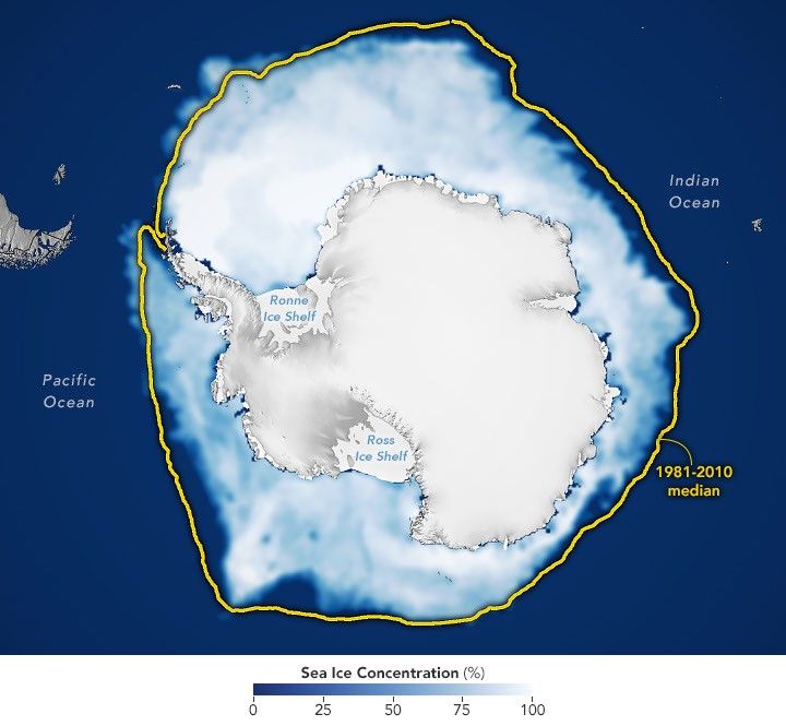
A map shows white Antarctic sea ice on September 14, 2026, the day it reached its annual maximum extent. The 1981–2010 median is outlined in yellow.
Antarctic sea ice reached its annual maximum extent on September 14, 2026—the third-lowest maximum in the satellite record.
NASA Earth Observatory/Michala Garrison

This story is an update to the Antarctic sea ice feature in our World of Change series tracking long-term change on Earth’s surface through satellite imagery.

Unlike the Arctic—an ocean basin surrounded by land—the Antarctic is a large continent surrounded by an ocean. Because of this geography, sea ice has more room to expand during the winter. However, that ice also stretches into warmer latitudes, leading to more melting in the summer. Antarctic sea ice usually peaks in September, around the end of the Southern Hemisphere’s winter, and retreats to a minimum in February.

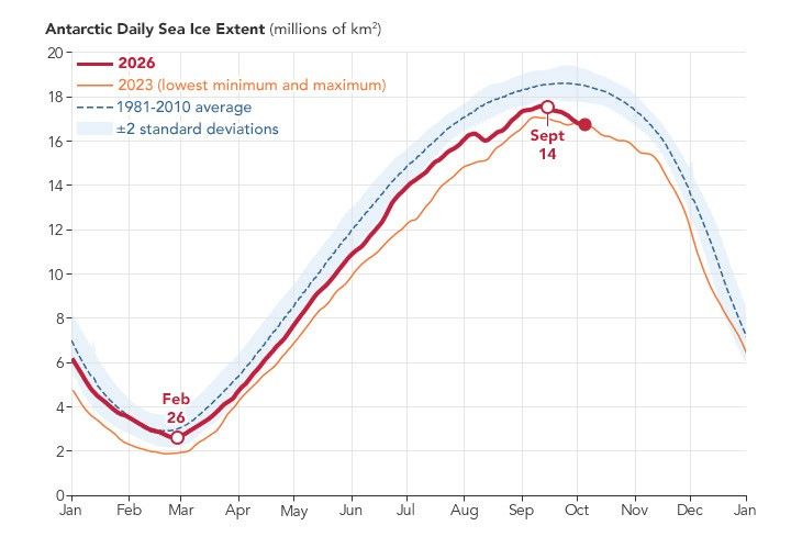
According to NASA and the National Snow and Ice Data Center (NSIDC), Antarctic sea ice in 2026 likely reached its annual maximum extent on September 14 (above). On that date, the ice covered an estimated 17.59 million square kilometers (6.79 million square miles), making it the third-lowest maximum on record.

The maps below show the average concentration of Antarctic sea ice for the month of September (left) and the following February (right) from 1990 to 2026. Opaque white areas indicate the highest concentrations, and dark blue areas are open water. The images include only areas where ice concentration was at least 15 percent, a threshold scientists commonly use to count an area as ice-covered in satellite data. Scientists refer to the total area of these regions as the “sea ice extent.”

1990-1991
1990-1991
1991-1992
1991-1992
1992-1993
1992-1993
1993-1994
1993-1994
1994-1995
1994-1995
1995-1996
1995-1996
1996-1997
1996-1997
1997-1998
1997-1998
1998-1999
1998-1999
1999-2000
1999-2000
2000-2001
2000-2001
2001-2002
2001-2002
2002-2003
2002-2003
2003-2004
2003-2004
2004-2005
2004-2005
2005-2006
2005-2006
2006-2007
2006-2007
2007-2008
2007-2008
2008-2009
2008-2009
2009-2010
2009-2010
2010-2011
2010-2011
2011-2012
2011-2012
2012-2013
2012-2013
2013-2014
2013-2014
2014-2015
2014-2015
2015-2016
2015-2016
2016-2017
2016-2017
2017-2018
2017-2018
2018-2019
2018-2019
2019-2020
2019-2020
2020-2021
2020-2021
2021-2022
2021-2022
2022-2023
2022-2023
2023-2024
2023-2024
2024-2025
2024-2025
Antarctic Sea Ice image pair showing 2025-2026
2025-2026

From Record Highs to Record Lows

From 1979 until 2014, total Antarctic sea ice increased by about 1 percent per decade. Whether the increase was a sign of meaningful change is uncertain because ice extents vary considerably from year to year around Antarctica. For three consecutive years, from 2012 to 2014, satellites observed new record highs for winter sea ice extent. These highs occurred while Arctic ice was in steep decline.

The climb came to an end in 2015, and significant decreases in sea ice around Antarctica started to occur in 2016. There have since been years with small rebounds, but overall, Antarctic sea ice coverage has largely remained lower than normal. Both the record low minimum and record low maximum occurred in 2023. Scientists will continue to observe the area each year to find out if the decline is part of a long-term change or a statistical fluctuation.

A line chart of Antarctic sea ice extent shows the 1981–2010 average as a blue dashed line, 2023 (the lowest minimum and lowest maximum on record) in orange, and 2026 in red.

Seeing Through the Clouds

To determine sea ice extent, scientists rely on satellites with passive microwave sensors that measure the microwave energy Earth naturally emits. Sea ice emits more of this energy than open water, so it stands out in microwave images. Because microwaves pass through clouds, the satellites can observe sea ice regularly, regardless of weather.

The record began in late 1978 with data collected by NASA’s Nimbus-7, followed by Defense Meteorological Satellite Program (DMSP) satellites starting in 1987, and by NASA’s Aqua satellite between 2002 and 2011. In 2025, scientists began using observations from the Japan Aerospace Exploration Agency’s GCOM-W satellite. 

NASA Earth Observatory images by Michala Garrison, using data from the National Snow and Ice Data Center.

Downloads

A map shows white Antarctic sea ice on September 14, 2026, the day it reached its annual maximum extent. The 1981–2010 median is outlined in yellow.

September 14, 2026

JPEG (682.33 KB)

References & Resources

You may also be interested in:

Stay up-to-date with the latest content from NASA as we explore the universe and discover more about our home planet.

Arctic Sea Ice Shrinks to Its 2026 Minimum
4 min read

Satellite records show Arctic sea ice covering less of the ocean in both winter and summer.

Article
A Changing World for Emperor Penguins
7 min read

Experts are analyzing decades of images from Landsat satellites for clues about how the iconic birds have responded to sea…

Article
Pink Penguin Guano Provides Diet Clues
3 min read

The color of Adélie penguin droppings reveals what the birds are eating, offering scientists a way to track how sea…

Article

Arctic Sea Ice Shrinks to Its 2026 Minimum

7 October 2026 at 00:00
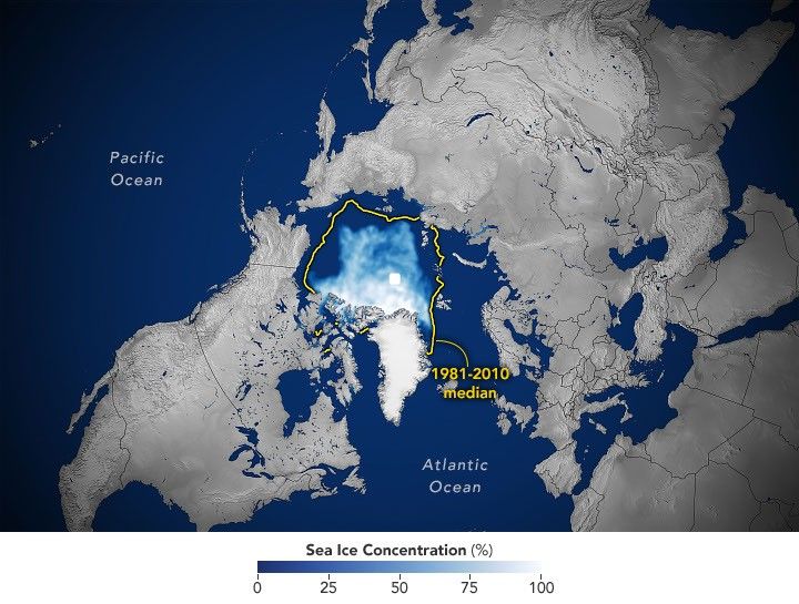
A map of the shows sea ice in September 2026 covering a smaller area than the 1981–2010 median, which is outlined in yellow.
Arctic sea ice reaches its annual minimum extent on September 12, 2026, tying several past years for the 10th-lowest minimum in the satellite record.
NASA Earth Observatory/Michala Garrison

This story is an update to the Arctic sea ice feature in our World of Change series, which tracks long-term change on Earth’s surface through satellite imagery.

A layer of frozen seawater caps the Arctic Ocean. This sea ice grows through the long polar winter, usually peaking in March, then melts through the summer to its annual low in September. It is a natural fluctuation that has persisted for millennia. But satellite records show the ice now covers less of the Arctic Ocean at its annual maximum and minimum than it did a few decades ago.

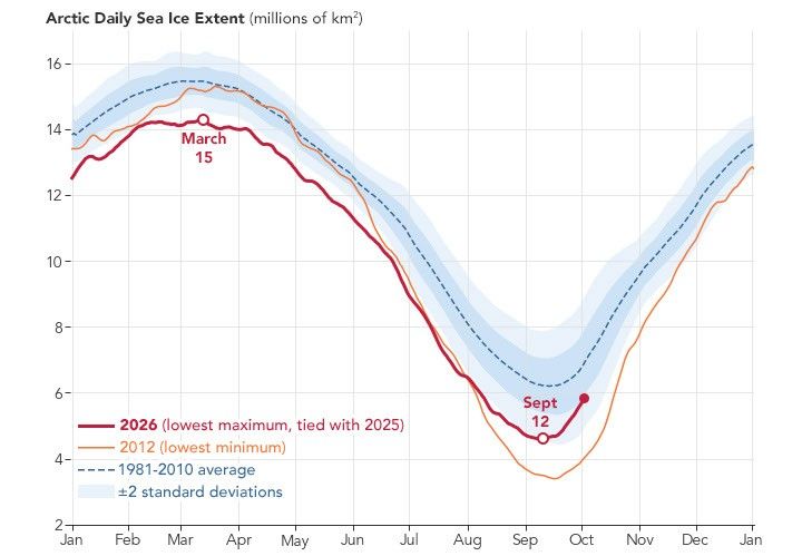
Sea ice in 2026 reached its annual minimum extent on September 12 (above), when it covered an estimated 4.6 million square kilometers (1.78 million square miles), according to NASA and the National Snow and Ice Data Center (NSIDC). That ties 2008, 2010, and 2025 for the 10th-lowest minimum in the satellite record.

The maps below pair each September since 1990 (left), around the ice’s annual minimum, with the following March (right), near its annual maximum, through March 2026.

1990-1991
1990-1991
1991-1992
1991-1992
1992-1993
1992-1993
1993-1994
1993-1994
1994-1995
1994-1995
1995-1996
1995-1996
1996-1997
1996-1997
1997-1998
1997-1998
1998-1999
1998-1999
1999-2000
1999-2000
2000-2001
2000-2001
2001-2002
2001-2002
2002-2003
2002-2003
2003-2004
2003-2004
2004-2005
2004-2005
2005-2006
2005-2006
2006-2007
2006-2007
2007-2008
2007-2008
Arctic Sea Ice image pair showing 2008-2009
2008-2009
2009-2010
2009-2010
2010-2011
2010-2011
2011-2012
2011-2012
2012-2013
2012-2013
2013-2014
2013-2014
2014-2015
2014-2015
2015-2016
2015-2016
2016-2017
2016-2017
2017-2018
2017-2018
2018-2019
2018-2019
2019-2020
2019-2020
2020-2021
2020-2021
2021-2022
2021-2022
2022-2023
2022-2023
2023-2024
2023-2024
Arctic Sea Ice image pair showing 2024-2025
2024-2025
2025-2026
2025-2026

Lower Lows, Thinner Ice

Scientists have used satellites to observe the annual growth and retreat of Arctic sea ice continuously since late 1978. While sea ice extent has declined overall during that time, the downward trend steepened in the 2000s and set off a run of record and near-record lows. Each of the past 20 summers, from 2007 through 2026, ranks among the 20 lowest minimum extents in the satellite record. The lowest occurred in September 2012.

More recently, the September sea ice extent has been relatively steady. Weather can make a big difference in how much ice melts from one summer to the next. For example, over the past decade, increased cloud cover has prevented sunlight from accelerating the melt, according to NASA scientists. Despite this recent plateau, the summer minimum remains well below the long-term average.

Across the Arctic, the ice that remains is younger and thinner. Observations show a decline in multiyear ice—that which survives at least one melt season—leaving an Arctic dominated by thinner first-year ice. Winter ice is also shrinking. The March 2026 maximum statistically tied the 2025 maximum for the lowest in the satellite record.

A line chart of Arctic sea ice extent shows the 1981–2010 average as a blue dashed line, 2012 (the record-low minimum year) in orange, and 2026 in red. The 2026 line stays below the average and peaks in March at a level that tied 2025 for the lowest maximum on record.

Cycles of natural variability such as the Arctic Oscillation are known to play a role in Arctic sea ice extent, but the decline observed throughout the satellite record cannot be explained by natural variability alone. Natural variability and rising global temperatures have worked together to melt greater amounts of Arctic sea ice. Scientists have projected an essentially ice-free Arctic could occur at least once before the middle of the 21st century.

Seeing Through the Clouds

To determine sea ice extent, scientists rely on satellites with passive microwave sensors that measure the microwave energy Earth naturally emits. Sea ice emits more of this energy than open water, so it stands out in microwave images. Because microwaves pass through clouds, the satellites can observe sea ice regularly, regardless of weather.

The record began in 1978 with data collected by NASA’s Nimbus-7, followed by Defense Meteorological Satellite Program (DMSP) satellites starting in 1987 and NASA’s Aqua satellite between 2002 and 2011. Starting in 2025, scientists began using observations from the Japan Aerospace Exploration Agency’s GCOM-W satellite. The white circle at the center of each image is the “pole hole,” north of which satellite sensors have historically been unable to collect data. The sea ice estimates assume that this hole is ice-filled.

NASA Earth Observatory images by Michala Garrison, using data from the National Snow and Ice Data Center.

Downloads

A map of the shows sea ice in September 2026 covering a smaller area than the 1981–2010 median, which is outlined in yellow.

September 12, 2026

JPEG (3.32 MB)

References & Resources

You may also be interested in:

Stay up-to-date with the latest content from NASA as we explore the universe and discover more about our home planet.

Arctic Melt Season Length Levels Off

4 min read

While the sea ice melt season has lengthened dramatically in most of the satellite era, the trend unexpectedly stabilized around…

Article

A Changing World for Emperor Penguins

7 min read

Experts are analyzing decades of images from Landsat satellites for clues about how the iconic birds have responded to sea…

Article

Pink Penguin Guano Provides Diet Clues

3 min read

The color of Adélie penguin droppings reveals what the birds are eating, offering scientists a way to track how sea…

Article

Uncovering the Valleys Hidden Below Greenland’s Ice

28 September 2026 at 00:00
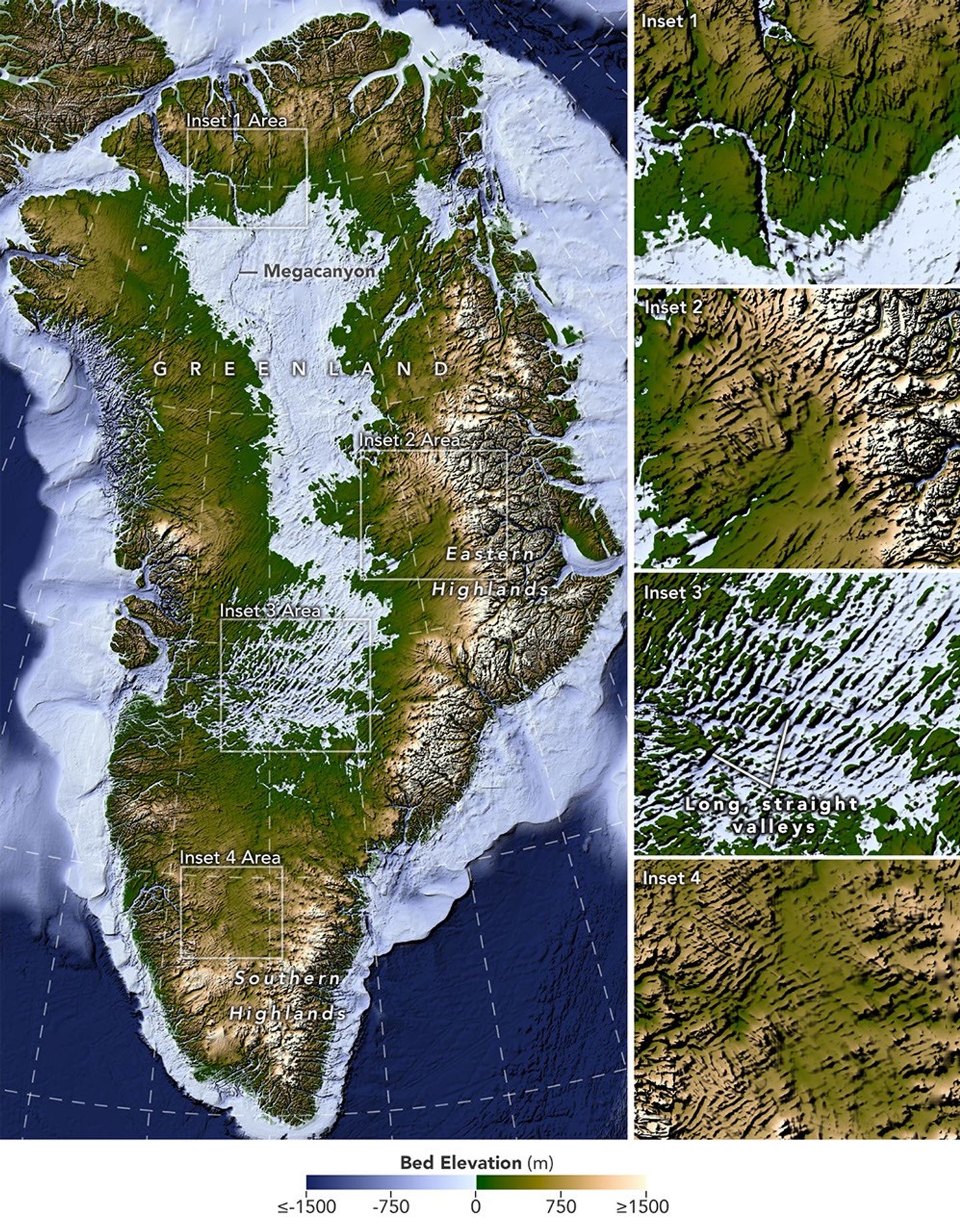
A large map on the left shows Greenland’s bedrock topography that lies below the ice sheet. A column of smaller maps on the right zooms in on several features, including long, straight valleys on the west-central part of the island. Other insets show a megacanyon, as well as valleys radiating outward from the highlands.
A newly developed method for mapping the bedrock beneath Greenland’s ice sheet reveals the island’s hidden topography. Among the most striking finds are long, straight valleys in the west-central region, some mapped for the first time and others extending farther inland than previously known (inset 3).
NASA Earth Observatory/Lauren Dauphin, based on data from Chartrand et al.

Greenland is capped with a vast ice sheet that spans 1.7 million square kilometers (656,000 square miles) and measures more than 3 kilometers (1.9 miles) at its thickest point. Below all this ice lies a landscape human eyes have never seen directly. But a newly developed method for mapping this hidden bedrock has produced the most detailed and accurate view of it yet.

The new map reveals an expansive network of valleys carved into the surface beneath the Greenland Ice Sheet. Many of the features formed well before most of the ice above them existed, offering new context for the island’s geologic history—and potentially helping scientists refine projections of the ice sheet’s future. Scientists described the newly mapped valleys in a NASA-led paper published in Geophysical Research Letters.

The map, shown above, was derived from a method called Ice Flow Perturbation Analysis. As ice flows over a valley or ridge, the topography leaves a faint signature on the ice surface. Satellites map the ice surface in fine detail, and scientists can use these subtle bumps and dips to infer the shape of the landscape buried below. The work aims to improve future versions of BedMachine Greenland, a high-resolution dataset of the terrain beneath the ice sheet.

Using the technique, researchers manually mapped 1,943 subglacial valleys beneath the Greenland Ice Sheet, about a third of which are newly identified. About half of the valleys included in BedMachine Greenland, primarily near the ice sheet’s edge, are now known to extend farther inland than that map indicates, in some cases by hundreds of kilometers.

Some aspects of the new map align with the current understanding of how Greenland’s landscapes formed. For instance, many of the valleys appear to begin in the southern and eastern highlands, where the ice sheet is thought to have first formed. Near the eastern highlands, the map reveals a mountain range beneath the ice, with interconnected valleys and relief that increases toward the coast. These alpine-style landforms may have survived under the ice since at least the Pliocene.

Other aspects of the topography are more puzzling. The analysis indicates numerous valleys, especially in the west-central region, that are long, straight, and consistently aligned in a southwest-northeast direction. This orientation suggests a tectonic influence, generating preferential pathways along which water could flow and valleys could form. “That’s a riddle to us,” said Joe MacGregor, a NASA cryospheric scientist and co-author of the study. “Greenland is justifiably usually treated as a rigid block of old rock that is simply translated as needed to accommodate the motion and interactions of other tectonic plates.”

Separately, the angles at which the valleys branch offer another insight into their origin. Their relatively wide branching angles suggest that surface water didn’t act alone; instead, a widespread groundwater network—seeping upward and eroding the surrounding rock—likely helped carve the valleys before the ice sheet formed.

Mapping these valleys matters for understanding the ice sheet, which has continued to dramatically reshape the landscape. Ice flow concentrates in valleys, where it forms glaciers that eventually calve into fjords at the periphery of the ice sheet. This creates a reinforcing cycle: ice funneling through a valley gets thicker, thicker ice flows faster, and faster flow carves the valley even deeper.

This carving power is especially evident along western Greenland. MacGregor likened it to the glacially incised landscape at Yosemite, with Greenland’s western coast resembling, as he put it, “El Capitan after El Capitan.”

Studying the valleys also matters for the ice sheet’s future. Because the relationship between ice flow and valleys is well understood, scientists expect that as the ice sheet retreats, flow will continue to concentrate wherever the valleys already are. “The better we understand the topography now,” MacGregor said, “the better sense we’ll have of what it will look like in the longer term—beyond the next decade or two—as faster ice flow propagates into Greenland’s interior.”

NASA Earth Observatory map by Lauren Dauphin using data from Chartrand et al. Story by Kathryn Hansen.

Downloads

A large map on the left shows Greenland’s bedrock topography that lies below the ice sheet. A column of smaller maps on the right zooms in on several features, including long, straight valleys on the west-central part of the island. Other insets show a megacanyon, as well as valleys radiating outward from the highlands.

Bedrock Map

JPEG (11.10 MB)

References & Resources

You may also be interested in:

Stay up-to-date with the latest content from NASA as we explore the universe and discover more about our home planet.

An Uncommon Drifter in the Denmark Strait

4 min read

A large iceberg, observed in summer 2026, had drifted more than 1,000 kilometers south from the northeastern Greenland bay where…

Article

A Bare Summer for Barnes Ice Cap

4 min read

The expanse of glacial ice on Canada’s Baffin Island lost its snow cover quickly and early in summer 2026, revealing…

Article

Pasterze Hangs on as Austria’s Largest Glacier

4 min read

One narrowing icefall remains the linchpin for the Alpine glacier—and it may not be long for this world.

Article
❌
❌