❌

Reading view

There are new articles available, click to refresh the page.

The Land of the Standing-Up Rocks

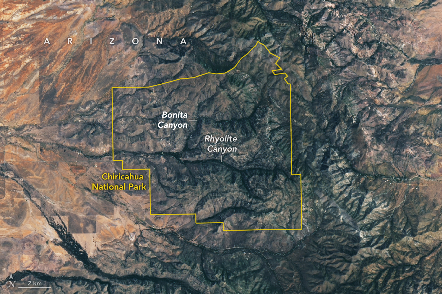
A satellite image shows Chiricahua National Park outlined in yellow amid mountainous terrain. Within the park, gray ridges are cut by green, vegetated canyons, two of which are labeled Bonita Canyon and Rhyolite Canyon. To the west, the land is flatter and redder with less vegetation.

Some 27 million years ago, a volcano in what’s now southeastern Arizona unleashed a spectacular series of eruptions, strewing more than 1,000 times as much volcanic material across the landscape as Mount St. Helens did in 1980.

The explosive eruptions blanketed the region, part of the Chiricahua Apache Nation’s traditional lands, with ash and pumice. Layered into this were massive pyroclastic flows that hardened into deposits of welded rhyolitic tuff that in some areas were nearly 1,600 feet (500 meters) thick, about three times the height of the Washington Monument. As the magma chamber emptied, the ground above it collapsed, leaving a gaping depression—the Turkey Creek caldera—that was roughly 12 miles (19 kilometers) wide and 4,900 feet (1,500 meters) deep.

An array of geologic processes, including erosion and weathering, gradually sculpted the welded layer of tuff into the collection of dramatic spires, hoodoos, and canyons that visitors to the caldera area encounter today.

The Apache called the area “The Land of the Standing-Up Rocks” for good reason. Hiking through Rhyolite Canyon or driving through Bonita Canyon means encountering a dizzying maze of rock pinnacles, some hundreds of feet tall. Others, like Big Balanced Rock, have surprisingly large boulders precariously perched on top. Meanwhile, those at Heart of Rocks and Massai Point are gathered into groups of hundreds.

The area was designated a national monument in 1924 to preserve its remarkable geology. In October 2026, it was redesignated as Chiricahua National Park (pronounced cheery-cow-ah). The OLI (Operational Land Imager) on Landsat 9 captured this cloud-free image of the new national park on July 2, 2026.

Individual rock spires are too small to distinguish, but the eroding rhyolitic tuff landscape appears gray. Stream valleys dense with trees and other vegetation, including Rhyolite Canyon and Bonita Canyon, snake across the landscape. With four biogeographic regions converging in the park—the Sonoran Desert, the Chihuahuan Desert, the Rocky Mountains, and the Sierra Madre—it is a haven of plant diversity.

Among the 1,000 species growing within the park’s varied desert, grassland, chaparral, deciduous forest, and coniferous forest ecosystems are agaves, prickly pear cacti, yuccas, manzanita, pine, fir, cypress, sycamore, juniper, and oak. The park’s location within the Chiricahua Mountains puts it among several “sky islands” in Arizona—isolated mountain ranges that emerge from the surrounding desert “sea.” According to the National Park Service, the range’s highest point (outside the park) rises 2,986 meters (9,795 feet) above sea level, more than 1,800 meters above the surrounding valley.

NASA Earth Observatory image by Lauren Dauphin, using Landsat data from the U.S. Geological Survey. Story by Adam Voiland.

Downloads

A satellite image shows Chiricahua National Park outlined in yellow amid mountainous terrain. Within the park, gray ridges are cut by green, vegetated canyons, two of which are labeled Bonita Canyon and Rhyolite Canyon. To the west, the land is flatter and redder with less vegetation.

July 2, 2026

JPEG (6.09 MB)

References & Resources

You may also be interested in:

Stay up-to-date with the latest content from NASA as we explore the universe and discover more about our home planet.
The Forested Floodplains of Congaree National Park
4 min read

The meandering Congaree River sustains towering forest ecosystems and fashions oxbow lakes as it shifts across its floodplain.
Article
Minute Man National Historical Park
3 min read

Sites relevant to the start of the American Revolutionary War are interspersed throughout the modern-day Boston metropolitan region.
Article
Colonial National Historical Park
2 min read

The colonial communities of “America’s historic triangle” played defining roles in the road to American independence.

Article

El Niño Then and Now

october 13, 1997
october 12, 2026
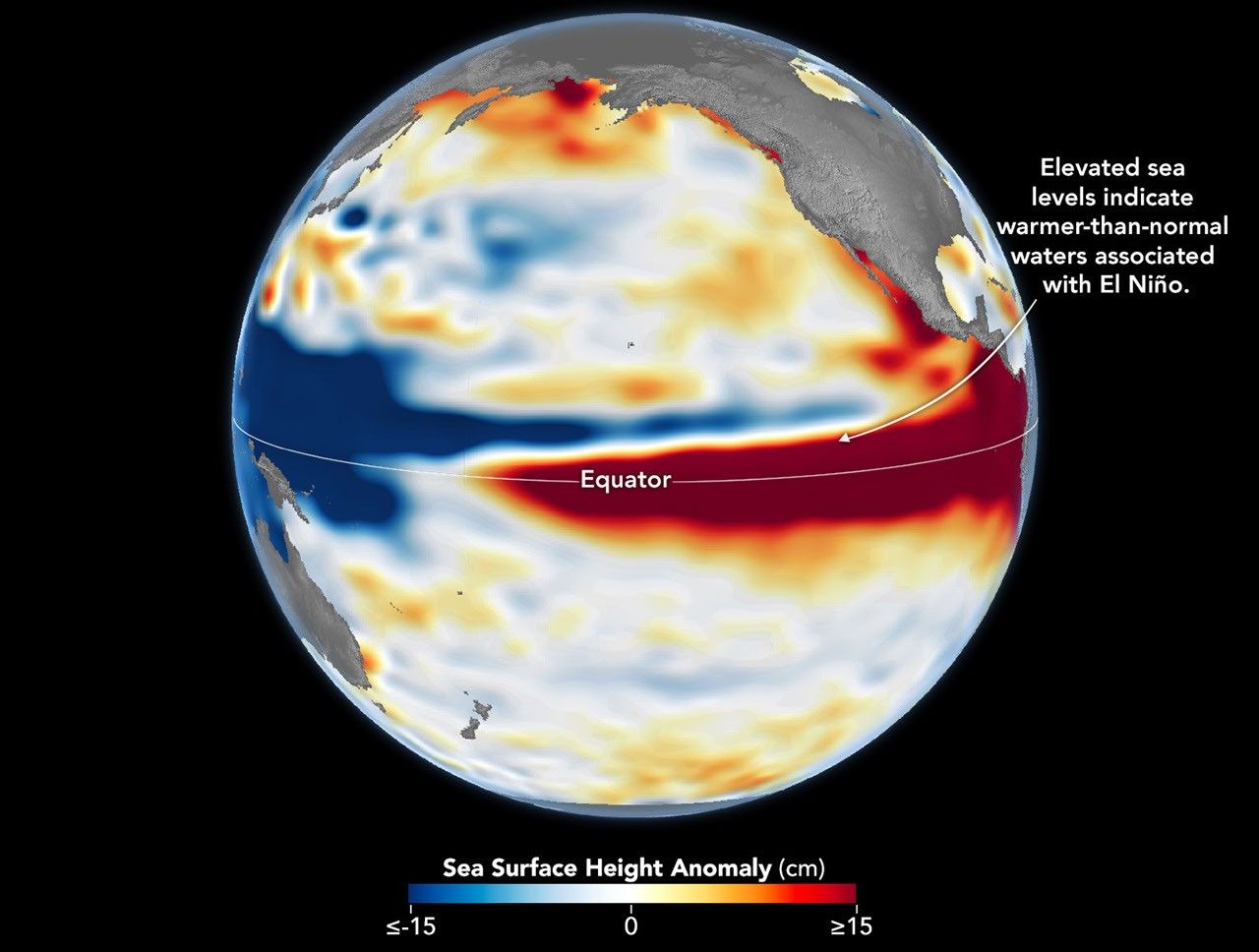
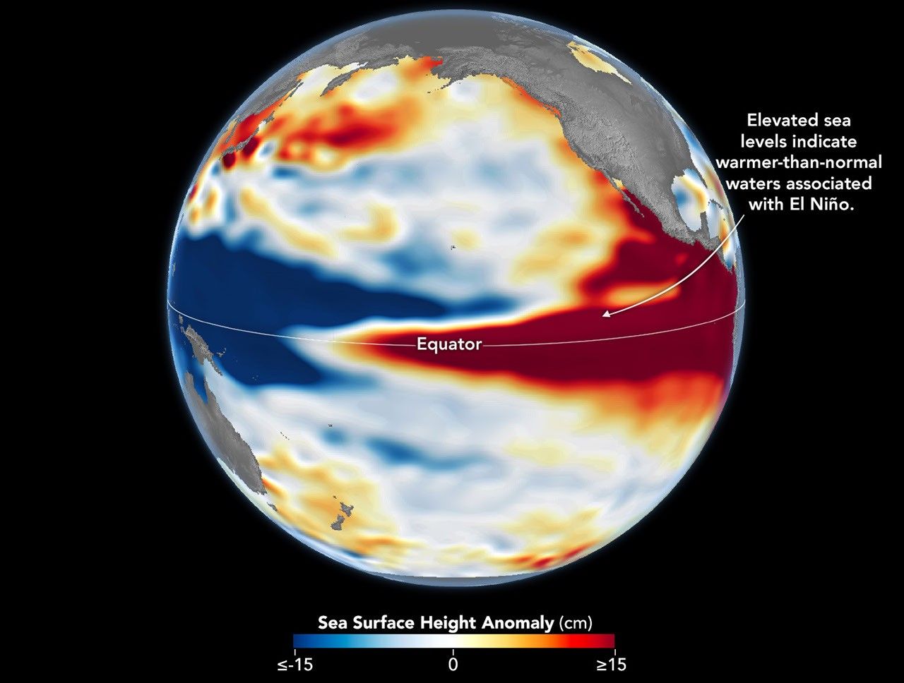
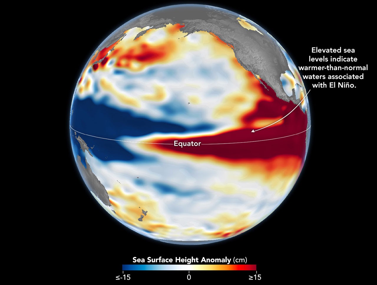
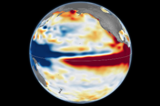
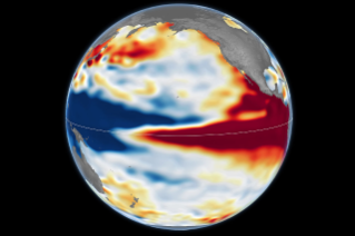
Side-by-side maps of the Pacific Ocean compare sea surface height anomalies in October 1997 (left) and October 2026 (right). In both, red areas of higher-than-normal sea surface height stretch across the central and eastern Pacific and reach South America.
Sea levels are higher than normal across the central and eastern equatorial Pacific in October 2026 (right), a hallmark of El Niño. The pattern closely resembles October 1997 (left), during another one of the strongest El Niño events in the satellite altimetry record.
NASA Earth Observatory / Lauren Dauphin
october 13, 1997
october 12, 2026

October 13, 1997 – October 12, 2026

Sea levels are higher than normal across the central and eastern equatorial Pacific in October 2026 (right), a hallmark of El Niño. The pattern closely resembles October 1997 (left), during another one of the strongest El Niño events in the satellite altimetry record. Maps by NASA Earth Observatory/Lauren Dauphin using altimetry data provided by NASA/JPL-Caltech.

El Niño is part of a natural climate pattern that occurs roughly every two to seven years, bringing warmer-than-normal water to parts of the equatorial Pacific. The most recent very strong El Niño events, in 1997-98 and 2015-16, upended weather patterns. Impacts spanned the planet, from fires in Indonesia and the Amazon, to crop failures due to drought in southern Africa, to heavy rain and coastal flooding in Southern California. The current El Niño rivals these past heavyweights.

Every El Niño grows from a feedback loop between the atmosphere and the ocean. Trade winds normally keep warm water piled up in the western Pacific, where it stands higher than in the east. When those winds weaken, that warm water begins to pulse eastward, which further weakens and sometimes reverses the winds, allowing even more warm water to move east. The cycle intensifies as waters continue to warm and pile up in the central and eastern Pacific.

But each El Niño has its own character, shaped by where in the Pacific the warmth builds and how the atmosphere responds. “The search for the ‘typical’ El Niño is very elusive,” said Josh Willis, project scientist for sea level missions at NASA’s Jet Propulsion Laboratory (JPL). “They’re all different in terms of where they land and how their impacts play out.”

Altimetry satellites can track those differences by measuring the height of the sea surface. Because water expands as it warms, higher-than-normal sea levels in the central and eastern equatorial Pacific signal the buildup of heat associated with El Niño. The maps above depict sea surface height anomalies across the Pacific Ocean on October 13, 1997 (left), and on October 12, 2026 (right). Data are from the TOPEX/Poseidon satellite and the Sentinel-6 Michael Freilich satellite, respectively, and were processed by scientists at JPL.

Shades of red indicate where sea levels were higher than average. Normal sea level conditions appear white, and lower areas are blue. Signals related to seasonal cycles and long-term trends have been removed to highlight sea level anomalies associated with El Niño and other short-term natural phenomena.

“What’s unique about altimetry is that we have a 35-year record from nearly identical satellites flying almost the same ground track, with each mission overlapping the next,” Willis said. “That lets us look back in time and compare this El Niño to what happened in 1997. And right now, this one is on track to be even bigger.”

Compared with the 1997-98 event, El Niño in 2026 came on much more suddenly. But as of October, the two events appear similar in character—the tilt of sea level (low in the west and high in the east) and high, warm water extending all the way to South America—so Willis thinks the impacts could be similar as well. In 1997-98, that meant, for instance, lots of rain in California and across the southern tier of the U.S.

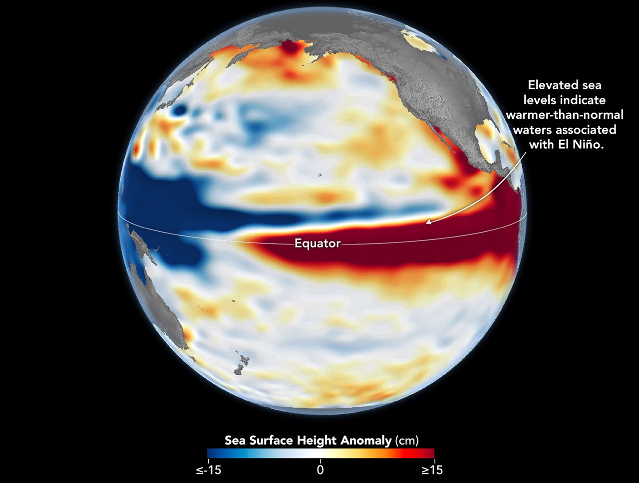
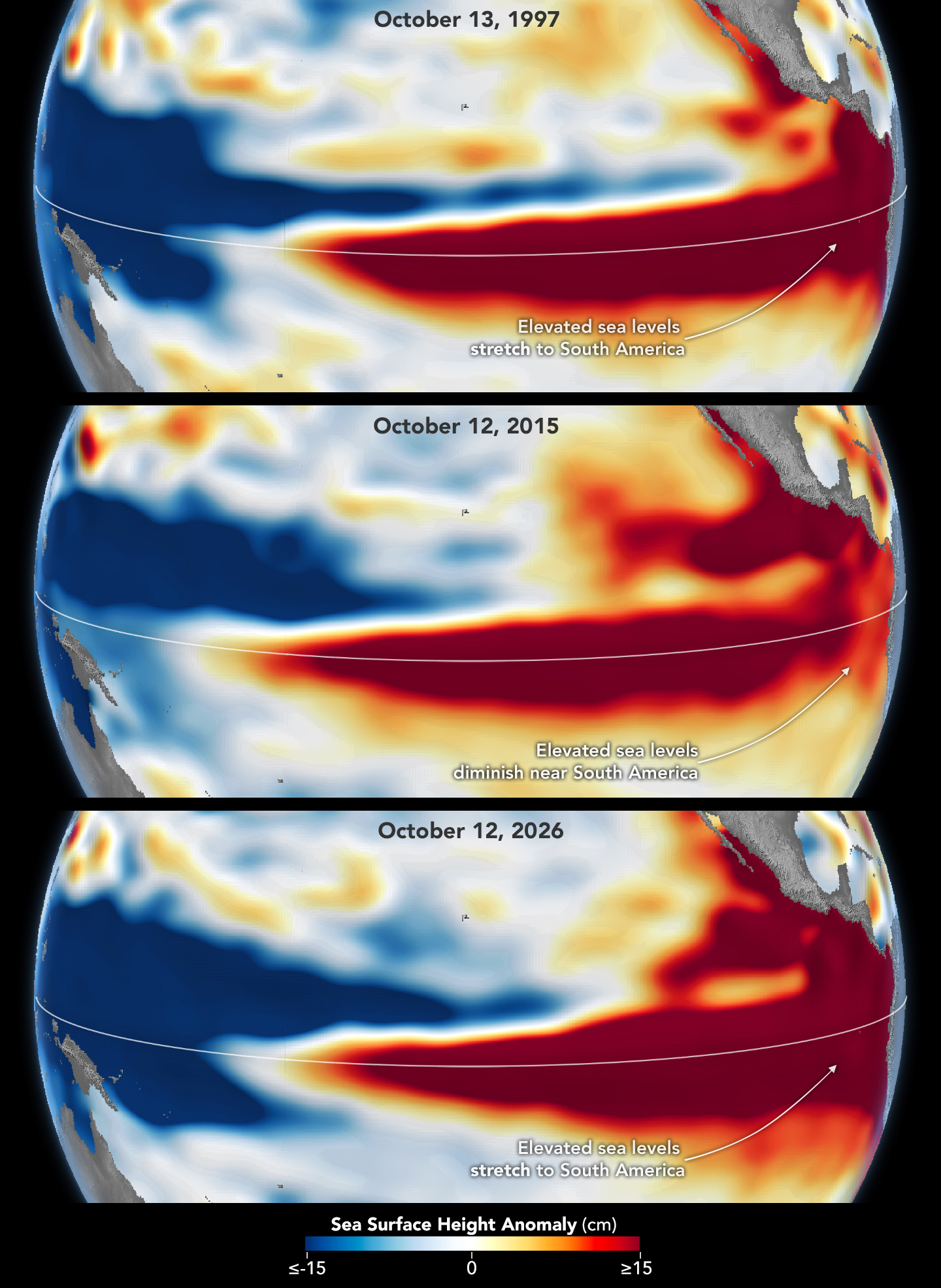
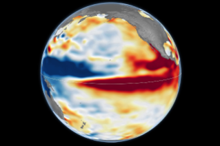
Three stacked maps of the Pacific Ocean compare sea surface height anomalies in October 1997 (top), October 2015 (middle), and October 2026 (bottom). In 1997 and 2026, dark red areas of exceptionally high sea surface height extend across the eastern Pacific and pile up against the coast of South America. In 2015, the dark red stays farther offshore and does not reach the coast.
The 2015-16 El Niño was also very strong, as elevated sea levels in October 2015 (middle) show. But its pattern differed from those in October 1997 (top) and October 2026 (bottom): less of the elevated water reached the coast of South America, which contributed to different weather patterns that year.

The 2015-16 El Niño was another heavy hitter but differed in its character. Sea surface height anomalies on October 12, 2015, based on altimetry data from the Jason-2 satellite, are shown above in context with maps from around the same time in 1997 and 2026. In 2015, the exceptionally warm, high water along the equator didn’t push up against South America to the extent it did in the other years. Rainfall impacts that winter concentrated more over Central America and the southeastern U.S., with significant flooding in Mexico.

NOAA’s El Niño outlook on October 8, 2026, called for an 83 percent chance of a strong-to-very strong El Niño through the first three months of 2027. But exactly how the impacts will play out in winter 2026-27 and beyond remains to be seen. Willis noted that El Niño’s influence propagates through a chaotic atmosphere, and the signal can get muddled as it extends beyond the tropics. “There’s always a bit of a dice roll here,” Willis said. “Just because this El Niño looks like 1997 doesn’t mean it will be exactly the same—it’s just our best guess at the moment.”

NASA Earth Observatory maps by Lauren Dauphin, using NASA-SSH altimetry data provided by Josh Willis, Severine Fournier, and Kevin Marlis, NASA/JPL-Caltech. Story by Kathryn Hansen.

Downloads

Side-by-side maps of the Pacific Ocean compare sea surface height anomalies in October 1997 (left) and October 2026 (right). In both, red areas of higher-than-normal sea surface height stretch across the central and eastern Pacific and reach South America.

October 13, 1997

JPEG (1.22 MB)

The 2015-16 El Niño was also very strong, as elevated sea levels in October 2015 show.

October 12, 2015

JPEG (1.21 MB)

Side-by-side maps of the Pacific Ocean compare sea surface height anomalies in October 1997 (left) and October 2026 (right). In both, red areas of higher-than-normal sea surface height stretch across the central and eastern Pacific and reach South America.

October 12, 2026

JPEG (1.24 MB)

References & Resources

You may also be interested in:

Stay up-to-date with the latest content from NASA as we explore the universe and discover more about our home planet.

El Niño Is Underway
4 min read

Satellite observations of sea surface height indicated that the 2026 event continued to strengthen in early June.

Article
How the Tide Turns at the Mouth of the Elbe
4 min read

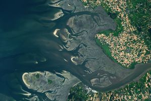
The ocean’s ebbs and flows reveal dynamic tidal flats and a well-traveled shipping route along the coast of Germany.

Article
El Niño Alters Marine Life in the Pacific
5 min read

Satellite measurements of chlorophyll at the sea surface signal shifts in the ocean’s nutrient supplies in mid-2026.

Article

Autumn Paints Poland’s Bieszczady Mountains

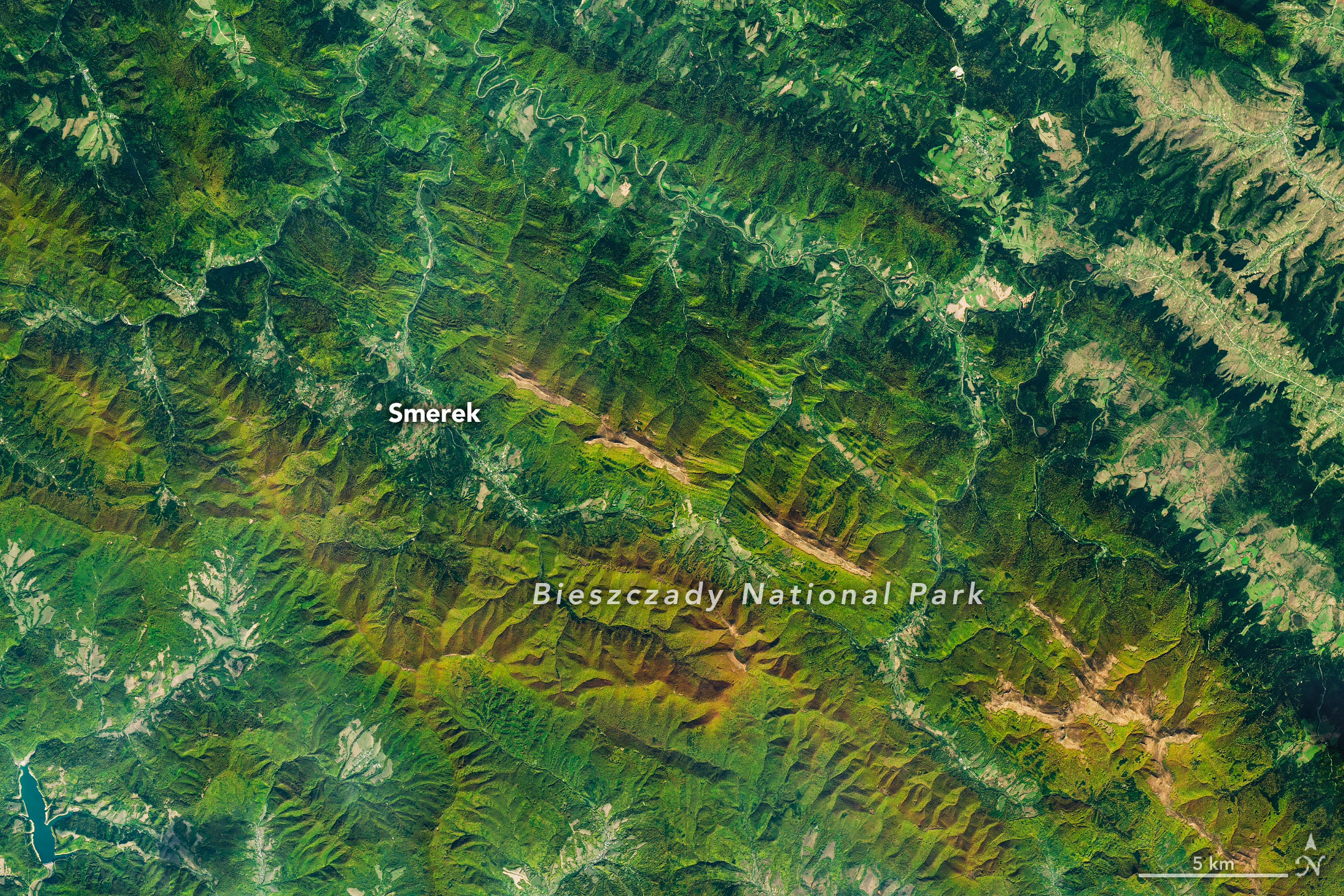
A satellite image of mountains in southeastern Poland in autumn. Green and orange forest covers parallel ridges running diagonally across the scene, and tan grasslands stretch along the highest crests.

As the air grows cooler and days shorter, brown bears prowl the Carpathian Mountains of southern Poland with the goal of fattening up ahead of winter hibernation. In a more conspicuous sign of autumn, beech and other deciduous trees blanketing the hillsides start to sport reds and golds. The seasonal transformation was underway in southeast Poland’s Bieszczady National Park on October 8, 2026, when the OLI (Operational Land Imager) on the NASA-USGS Landsat 9 satellite captured this image.

European beech (Fagus sylvatica) dominates the area’s forests, with other species such as sycamore maple (Acer pseudoplatanus) also contributing to vibrant color in the fall. Dropping air temperatures and waning daylight cause these trees to curtail the production of chlorophyll, the molecule that plants use to synthesize food. Without it, the leaves’ green pigments fade, allowing the yellows and reds of other pigments to show through.

A descendent of ice-age survivors, the European beech has persisted across millennia in a range of climates. After the glaciers retreated, beech forests spread northward across the European continent from isolated refugia in the Carpathians, Alps, and other mountain ranges, and played a crucial role in reforesting the previously ice-covered land. Portions of Bieszczady National Park are included within UNESCO’s network of ancient and primeval beech forests spanning 18 countries.

Expansive as their footprint across Europe may be, beech forests reach only so high in elevation—about 1,000 to 1,260 meters (3,300 to 4,100 feet)—in this area. Above that is the realm of the polonina, a Slavic term for subalpine meadow, consisting of open grasslands and shrubby thickets of rowan (mountain ash), willows, and green alder. Patches of polonina stretch across ridge tops to the east-southeast of Smerek and appear tan, having lost their summer greenness.

The Bieszczady Mountains are renowned not only for forests and mountain meadows but also for charismatic wildlife. European bison, once extinct in the wild, were reintroduced to the area in the 1960s and now roam the hills by the hundreds, according to recent surveys. Additionally, populations of brown bears and Eurasian lynx find refuge and ample food sources in the forests.

NASA Earth Observatory image by Michala Garrison, using Landsat data from the U.S. Geological Survey. Story by Lindsey Doermann.

Downloads

A satellite image of mountains in southeastern Poland in autumn. Green and orange forest covers parallel ridges running diagonally across the scene, and tan grasslands stretch along the highest crests.

October 8, 2026

JPEG (16.00 MB)

References & Resources

You may also be interested in:

Stay up-to-date with the latest content from NASA as we explore the universe and discover more about our home planet.

The Forested Floodplains of Congaree National Park
4 min read

The meandering Congaree River sustains towering forest ecosystems and fashions oxbow lakes as it shifts across its floodplain.

Article
Minute Man National Historical Park
3 min read

Sites relevant to the start of the American Revolutionary War are interspersed throughout the modern-day Boston metropolitan region.

Article
Colonial National Historical Park
2 min read

The colonial communities of “America’s historic triangle” played defining roles in the road to American independence.

Article

An Impact Structure With Legs

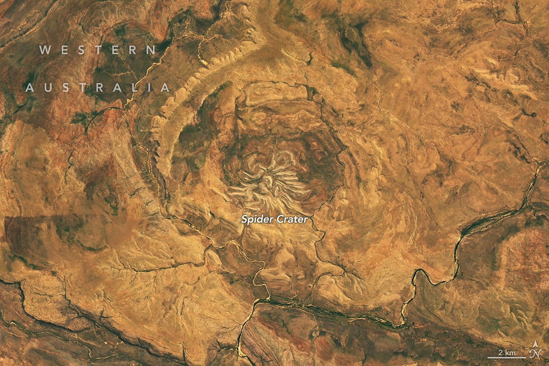
Several short, light-colored rocky ridges radiate out from a central point amid an orange and tan desert landscape.

Editor’s Note: Today’s story is the answer to the October Puzzler.

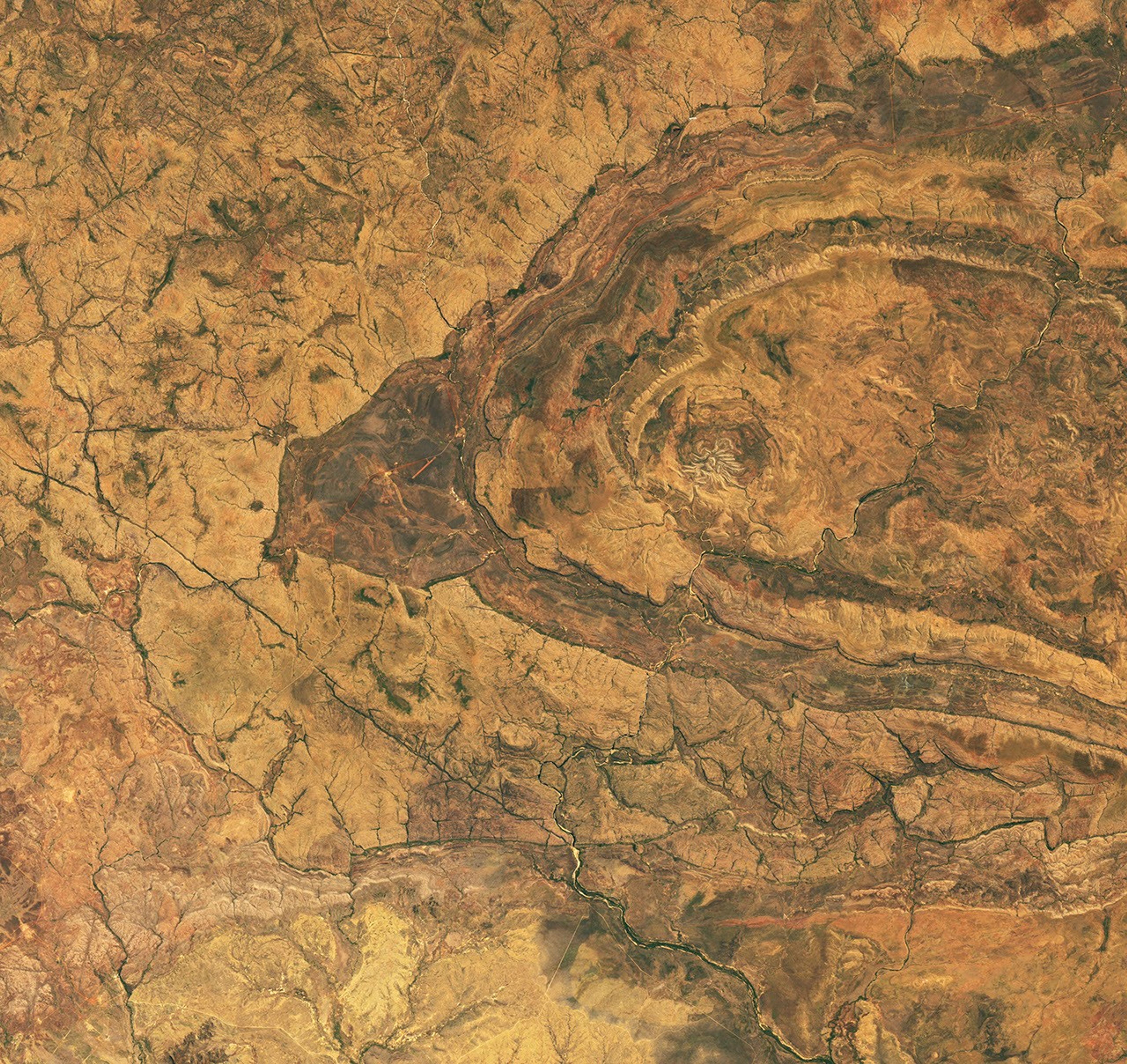
From above, the mere appearance of a curious geologic feature in Western Australia is enough to cause a fright. The aptly named Spider Crater, the product of a meteorite impact followed by hundreds of millions of years of erosion, sprawls across the landscape in the country’s Kimberley region.

The OLI (Operational Land Imager) on the NASA-USGS Landsat 9 satellite captured this image of the crater on September 20, 2026. The full impact structure has an oval shape measuring about 13 kilometers by 11 kilometers (8 miles by 7 miles), with the spiderlike central portion measuring about 4 kilometers (2.5 miles) across.

Geologists believe the unusual arachnoid pattern is the remnant of a central uplift, the raised portion of the crater floor that formed in the rebound of the initial impact shock. The light-colored “legs” are sandstone ridges that have endured while other rock layers in the impact zone have eroded away.

For decades after the feature’s discovery, scientists struggled to weave a tale about its formation. Some proposed it had a volcanic past. But with some legwork in the field, geologists identified telltale signs of a past impact: fan-shaped fractures called shatter cones. These fractures form only when intense shock waves travel through rock, and they are ubiquitous in Spider Crater’s central dome.

Scientists have subsequently performed lab analyses of shocked quartz and zircon crystals from the sandstone, which can help them reconstruct the angle of the meteorite’s impact. The date of the impact is uncertain, but estimates based on rocks in the region place it between about 900 million and 600 million years ago—making Spider Crater a creature of the late Precambrian.

NASA Earth Observatory image by Michala Garrison, using Landsat data from the U.S. Geological Survey. Story by Lindsey Doermann.

Downloads

Several short, light-colored rocky ridges radiate out from a central point amid an orange and tan desert landscape.

September 20, 2026

JPEG (23.76 MB)

References & Resources

You may also be interested in:

Stay up-to-date with the latest content from NASA as we explore the universe and discover more about our home planet.

An Accidental Impact Crater Discovery 
5 min read

An amateur astronomer scouting online satellite maps for campsites in Quebec found an impact crater instead.

Article
Boom Year for Desert Blooms
3 min read

Carpets of wildflowers burst from arid, ochre-colored land in Western Australia following winter rains.

Article
Moon-Like Madagascar
3 min read

A bright lens of anorthosite, a rock type prevalent on the lunar surface, is cradled within sheared rocks in the…

Article

Uncovering the Valleys Hidden Below Greenland’s Ice

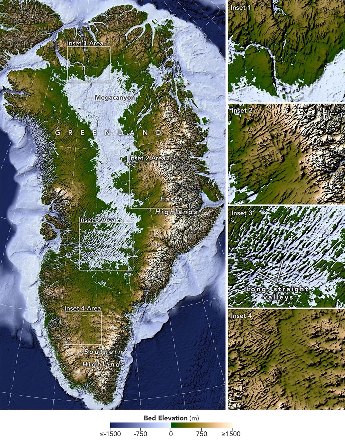
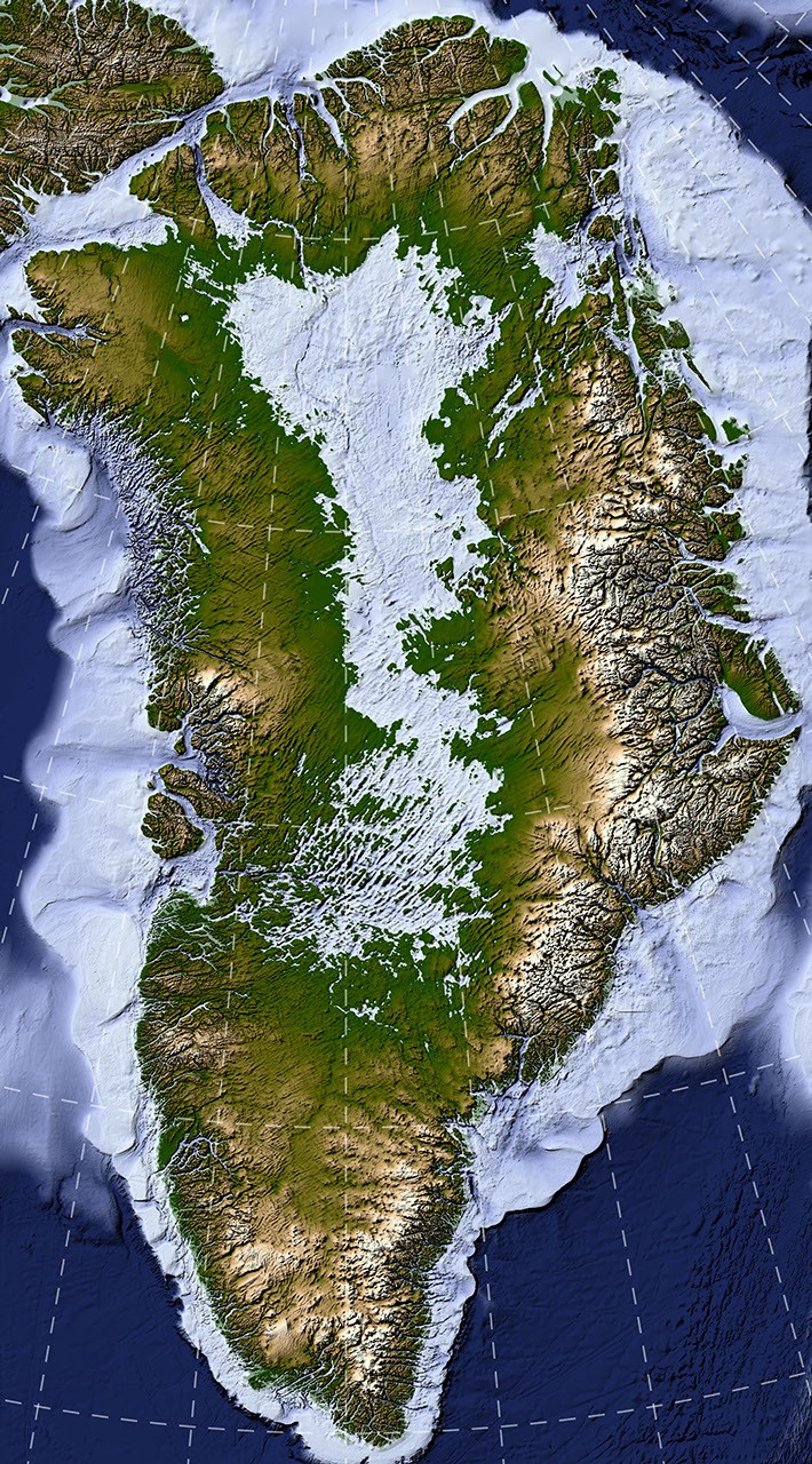
A large map on the left shows Greenland’s bedrock topography that lies below the ice sheet. A column of smaller maps on the right zooms in on several features, including long, straight valleys on the west-central part of the island. Other insets show a megacanyon, as well as valleys radiating outward from the highlands.
A newly developed method for mapping the bedrock beneath Greenland’s ice sheet reveals the island’s hidden topography. Among the most striking finds are long, straight valleys in the west-central region, some mapped for the first time and others extending farther inland than previously known (inset 3).
NASA Earth Observatory/Lauren Dauphin, based on data from Chartrand et al.

Greenland is capped with a vast ice sheet that spans 1.7 million square kilometers (656,000 square miles) and measures more than 3 kilometers (1.9 miles) at its thickest point. Below all this ice lies a landscape human eyes have never seen directly. But a newly developed method for mapping this hidden bedrock has produced the most detailed and accurate view of it yet.

The new map reveals an expansive network of valleys carved into the surface beneath the Greenland Ice Sheet. Many of the features formed well before most of the ice above them existed, offering new context for the island’s geologic history—and potentially helping scientists refine projections of the ice sheet’s future. Scientists described the newly mapped valleys in a NASA-led paper published in Geophysical Research Letters.

The map, shown above, was derived from a method called Ice Flow Perturbation Analysis. As ice flows over a valley or ridge, the topography leaves a faint signature on the ice surface. Satellites map the ice surface in fine detail, and scientists can use these subtle bumps and dips to infer the shape of the landscape buried below. The work aims to improve future versions of BedMachine Greenland, a high-resolution dataset of the terrain beneath the ice sheet.

Using the technique, researchers manually mapped 1,943 subglacial valleys beneath the Greenland Ice Sheet, about a third of which are newly identified. About half of the valleys included in BedMachine Greenland, primarily near the ice sheet’s edge, are now known to extend farther inland than that map indicates, in some cases by hundreds of kilometers.

Some aspects of the new map align with the current understanding of how Greenland’s landscapes formed. For instance, many of the valleys appear to begin in the southern and eastern highlands, where the ice sheet is thought to have first formed. Near the eastern highlands, the map reveals a mountain range beneath the ice, with interconnected valleys and relief that increases toward the coast. These alpine-style landforms may have survived under the ice since at least the Pliocene.

Other aspects of the topography are more puzzling. The analysis indicates numerous valleys, especially in the west-central region, that are long, straight, and consistently aligned in a southwest-northeast direction. This orientation suggests a tectonic influence, generating preferential pathways along which water could flow and valleys could form. “That’s a riddle to us,” said Joe MacGregor, a NASA cryospheric scientist and co-author of the study. “Greenland is justifiably usually treated as a rigid block of old rock that is simply translated as needed to accommodate the motion and interactions of other tectonic plates.”

Separately, the angles at which the valleys branch offer another insight into their origin. Their relatively wide branching angles suggest that surface water didn’t act alone; instead, a widespread groundwater network—seeping upward and eroding the surrounding rock—likely helped carve the valleys before the ice sheet formed.

Mapping these valleys matters for understanding the ice sheet, which has continued to dramatically reshape the landscape. Ice flow concentrates in valleys, where it forms glaciers that eventually calve into fjords at the periphery of the ice sheet. This creates a reinforcing cycle: ice funneling through a valley gets thicker, thicker ice flows faster, and faster flow carves the valley even deeper.

This carving power is especially evident along western Greenland. MacGregor likened it to the glacially incised landscape at Yosemite, with Greenland’s western coast resembling, as he put it, “El Capitan after El Capitan.”

Studying the valleys also matters for the ice sheet’s future. Because the relationship between ice flow and valleys is well understood, scientists expect that as the ice sheet retreats, flow will continue to concentrate wherever the valleys already are. “The better we understand the topography now,” MacGregor said, “the better sense we’ll have of what it will look like in the longer term—beyond the next decade or two—as faster ice flow propagates into Greenland’s interior.”

NASA Earth Observatory map by Lauren Dauphin using data from Chartrand et al. Story by Kathryn Hansen.

Downloads

A large map on the left shows Greenland’s bedrock topography that lies below the ice sheet. A column of smaller maps on the right zooms in on several features, including long, straight valleys on the west-central part of the island. Other insets show a megacanyon, as well as valleys radiating outward from the highlands.

Bedrock Map

JPEG (11.10 MB)

References & Resources

You may also be interested in:

Stay up-to-date with the latest content from NASA as we explore the universe and discover more about our home planet.

An Uncommon Drifter in the Denmark Strait

4 min read

A large iceberg, observed in summer 2026, had drifted more than 1,000 kilometers south from the northeastern Greenland bay where…

Article

A Bare Summer for Barnes Ice Cap

4 min read

The expanse of glacial ice on Canada’s Baffin Island lost its snow cover quickly and early in summer 2026, revealing…

Article

Pasterze Hangs on as Austria’s Largest Glacier

4 min read

One narrowing icefall remains the linchpin for the Alpine glacier—and it may not be long for this world.

Article
❌